IBDP. AI. HL. Graph Theory. Travelling Salesman

The Travelling Salesman Problem is: A travelling salesman leaves his home town, visits all the towns in the district, then returns home. How should he do this so that the distance he travels is minimised?

Hence we are interested in a journey along the edges of a graph starting and finishing at the same vertex and visiting every vertex in between.

We first consider complete graphs with the Euclidean property that the direct route between any two vertices is the shortest route between them. For this we consider the classical Travelling Salesman Problem: For a given weighted complete graph, find a Hamiltonian cycle of least weight.

For instance, suppose the salesman lives in town A and wants to visit each of the towns exactly once before returning to A. The distances are given in kilometres.

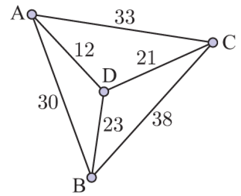
The Hamiltonian cycles that start and finish at A are:

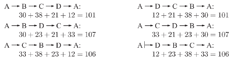
Notice that the three cycles on the right are simply the reverse of those on the left, so we didn’t need to show these calculations.

This method of solving the TSP is useful for small graphs, but becomes impractical as the size increases. There are algorithms however that we can apply to determine the upper and lower bounds for m, the weight of the minimum weight Hamiltonian cycle.

Finding an Upper Bound

For a complete graph with at least 3 vertices we can visit any unvisited vertex whenever we like, and once all the vertices have been visited we can return to the starting vertex immediately. We are therefore guaranteed that a Hamiltonian cycle exists for all complete graphs k_n, $n \geq 3$ . For this special case a Hamiltonian cycle can be found using the nearest neigbour algorithm:

Step 1: Choosing a starting vertex.
Step 2: Follow the edge of least weight to an unvisited vertex. If there is more than one such edge, choose one at random.
Step 3: Repeat “Step 2” until all vertices have been visited.
Step 4: Return to the starting vertex by adding the corresponding edge.

The sequence of visited vertices is a Hamiltonian cycle. It will be of low, but not necessarily minimum weight. Its weight hence serves as an upper bound for m.

Worked Example 1

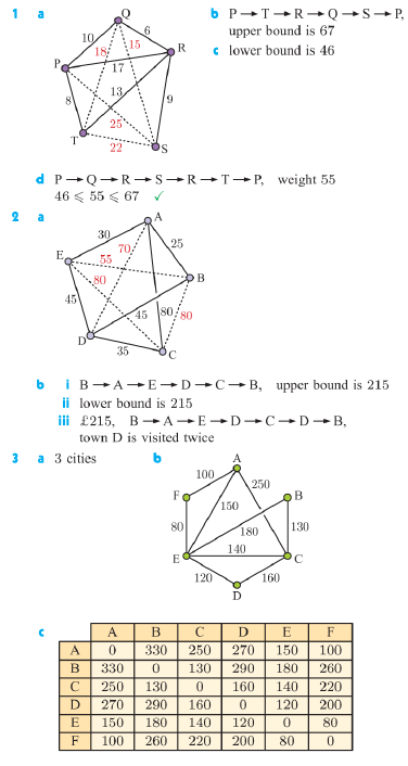
Consider the weighted complete graph below:

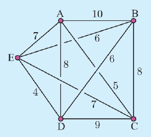
Use the nearest neighbour algorithm starting at A to find a Hamiltonian cycle for the graph. Hence find an upper bound for the TSP.

Finding a lower bound

Let G be a weighted complete graph on the n vertices V₁, V₂, … ,V_n. The vertices are labelled so that V₁ -> V₂ -> … -> V_n -> V₁ is the Hamiltonian cycle with minimum weight m and is therefore the solution to the TSP for G.

So m = weight of V₁V₂ + weight of V₁V_n + weight of path V₂ -> V₃ -> … -> V_n.

Now consider the graph H which is G with vertex V₁ removed and all edges connected to V₁ removed. H is the complete graph on the n-1 vertices V₂, V₃, …, V_n.

The path V₂ -> V₃ -> … -> V_n is a spanning tree of H, but not necessarily a minimum spanning tree.

Hence, the weight of path V₂ -> V₃ -> … -> V_n $\geq$ weight of a minimum spanning tree of H.

So m $\geq$ weight of V₁V₂ + weight of V₁V_n + weight of a minimum spanning tree of H.

This observation is the basis for the deleted vertex algorithm, which gives a lower bound for the TSP.

Step 1: Delete a vertex, together with all edges connected to it, from the original graph.
Step 2: Find the minimum spanning tree for the remaining graph.
Step 3: Add to the length of the minimum spanning tree, the lengths of the two shortest deleted deges.

The resulting value is a lower bound for m, the minimum weight for the solution to the TSP.

Worked Example 2

Below is the same graph as in worked example 1:

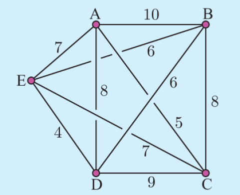
Apply the deleted vertex algorithm by deleting vertex A. Hence obtain a lower bound for the TSP.

The Practical TSP

Now let’s consider the graph below which shows roads between towns and the time it takes in minutes to travel along them:

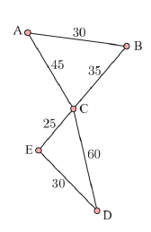
Note that this graph is neither complete nor Hamiltonian. It is not possible to visit every town and return to the starting point without visiting some towns more than once. It is also faster to travel from C to D via E than it is to travel directly from C to D. This may be because the road connecting C and D is very windy, or of poor quality. In such a case it may be preferable to take the faster route through E, even if this means visiting E more than once.

Practical TSP: For a given weighted graph, find the route of least weight which starts and finishes at the same vertex and visits each vertex at least once.

In the graph above, the solution to the practical TSP is the route A -> B -> C -> E -> D -> E -> C -> A, which takes 220 minutes. Notice that C and E are visited twice.

A practical TSP can be converted into a classical TSP by turning the graph into a complete Euclidean graph by adding or replacing edges to show the least weight between vertices.

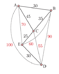
For instance, the fastest route between A and E above is 45 + 25 = 70 minutes, and the fastest route between C and D is 25 + 30 = 55 minutes.

Solving the classical TSP for the transformed graph is equivalent to solving the practical TSP for the original graph.

Worked Example 3

Consider the graph below:

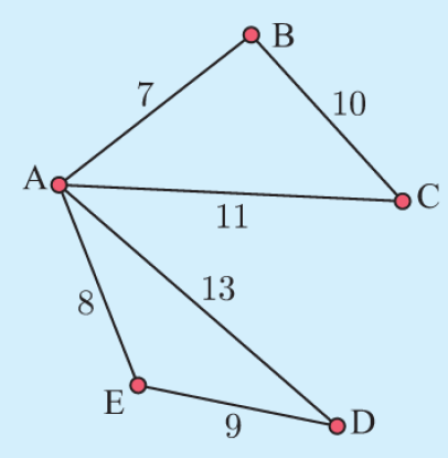
Complete the graph with edges showing the shortest distance between vertices;
Use the nearest neighbour algorithm starting at vertex A to find an upper bound for the TSP;
Use the deleted vertex algorithm with vertex A deleted to find a lower bound for the TSP.

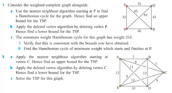
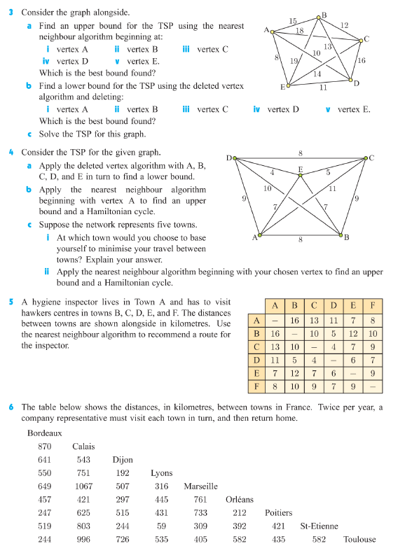
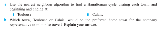
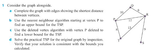
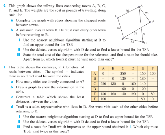
Exercise