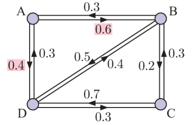
Below is a directed weighted graph showing the movement of buses between cities. The weights of the edges indicate probabilities, e.g. from city A 60% of the buses travel to city B and 40% to city D.

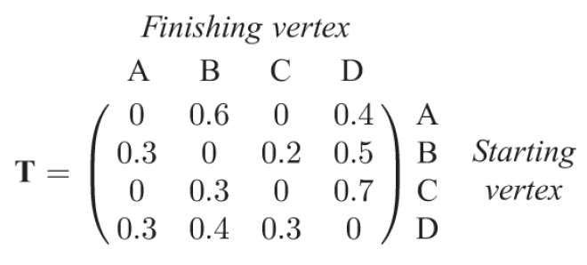
We can construct a transition matrix for this graph, as shown below. As with the adjacency matrices, the rows represent the starting vertices and the columns represent the finishing vertices.

The transition matrix is useful because it allows us to study the movement of the buses in the future. For example, consider T³ below:

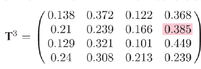
The shaded element tells us that a bus currently at B has probability 0.385 of being at D in three stops’ time.

The initial state matrix s₀ must now be written as a row matrix rather than a column matrix and we must premultiply Tⁿ by s₀ to find s_n. For example, if a bus is initially at B, then s₀ = (0 1 0 0) and s₁ = s₀T = , so, one stop from now, a bus currently at B has probability 0.3 of being at A, probability 0.2 of being at C and probability 0.5 of being at D.

Exercise

Answers