IBDP. AI. HL. DEs. Phase Portraits

Let’s start by considering the Lotka-Volterra Predator-Prey Model. This was originally formulated to describe chemical reactions but was extended by Kolmogorov to problems in mathematical biology.

The model considers populations of prey, x, and predators, y, as they change over time, t.

Imagine a population of y lions and x zebras as it varies over time. Because the two populations interact, the changes in each of their population is affected by both species. They can be modeled by the following two differential equations:

$\frac{dx}{dt} = 30x - xy$
$\frac{dy}{dt} = 0.015xy - 30y$

Reflect on the following questions:

What constraints are there on the variables x and y?
Suppose there are no predators, so y = 0:
- Find $\frac{dy}{dt}$ and interpret this value.
- Find $\frac{dx}{dt}$ . Explain what will happen to the population of zebras.
Suppose there are no prey, so x = 0:
- Find $\frac{dx}{dt}$ and interpret this value.
- Find $\frac{dy}{dt}$ . What will happen to the population of lions and why?
If x = 0 and y = 0 simultaneously, then both the populations are extinct and clearly $\frac{dx}{dt}$ and $\frac{dy}{dt}$ must both be zero. Can you find another pair of values (x,y) such that $\frac{dx}{dt}$ and $\frac{dy}{dt}$ equal zero? What does this mean for the two populations?
How can we find the solutions to these differential equations and hence know what will happen to the populations over time?

When we have simultaneous DEs, we say the DEs are coupled.

We define an equilibrium point as any point at which $\frac{dx}{dt} = \frac{dy}{dt} = 0$ . Once a system reaches such a point it will stay in equilibrium forever.

Velocity, for instance, can be given in its perpendicular components as:

$\frac{dx}{dt} = f_1 (x,y)$
$\frac{dy}{dt} = f_2 (x,y)$

The solution to the differential equations will be the parametric equations x(t) and y(t), showing position at time t. To fully specify x(t) and y(t) we would need an initial point (x₀,y₀).

Given a coupled system of DEs, we can give for any point in space (x,y), a trajectory vector $\begin{pmatrix} \frac{dx}{dt} \\ \frac{dy}{dt} \end{pmatrix}$

We can construct a diagram called a phase portrait, by drawing the appropriate vectors at each point in a Cartesian grid. Following the vector arrows from any point on the grid generates the trajectory or solution curve.

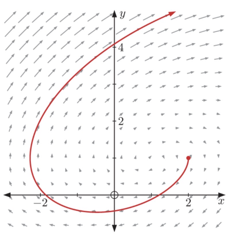
The diagram below shows the phase portrait for the coupled system of DEs:

$\frac{dx}{dt} = 2y - 2$
$\frac{dy}{dt} = y - x$ , along with the trajectory from (2,1).

Worked Example – Phase Portrait

The diagram below shows the phase portrait for the coupled system of DEs:

$\frac{dx}{dt} = y - \frac{1}{2} x$
$\frac{dy}{dt} = sin \pi x$

(a) Calculate $\begin{pmatrix} \frac{dx}{dt} \\ \frac{dy}{dt} \end{pmatrix}$ at the point:

(i.) (1,-1)
(ii) ( $\frac{1}{2}$ ,1)
Explain how these verctors are observed on the phase portrait.

(b) Illustrate the solution curves with the following initial points on the phase portrait:

(i) (2,0)
(ii) ( $- \frac{3}{2}$ , $\frac{1}{2}$ )
(iii) ( 2 , $- \frac{3}{2}$ )

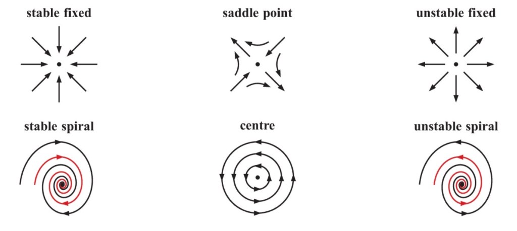
Equilibrium points

Equilibrium points can be classified according to the behaviour of the phase portrait around them, as illustrated below:

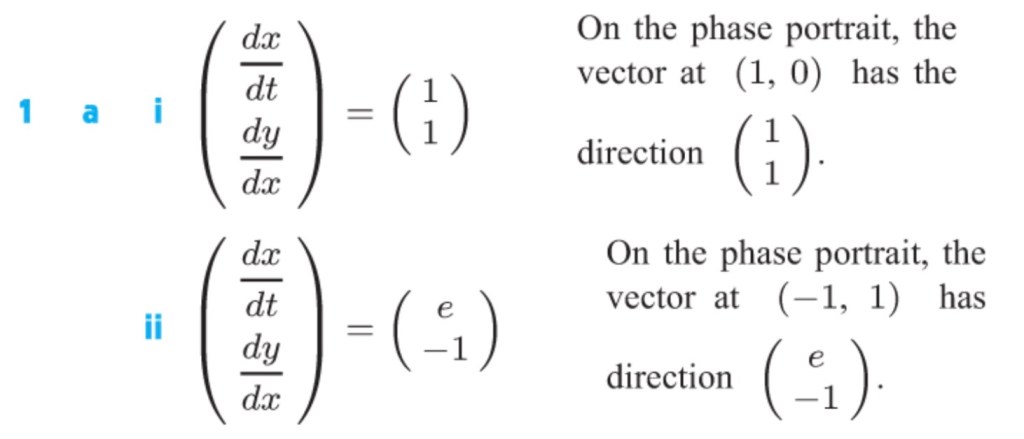
Exercise

The phase portrait is shown below for the coupled system of DEs:
- $\frac{dx}{dt} = e^y$
- $\frac{dy}{dt} = x$

(a) Calculate at the point:
- (i) (1,0)
- (ii) (-1,1)
- Explain how these vectors are observed on the phase portrait.
(b) Illustrate the solution curves with the following initial points on the phase portrait:
- (i) (-2, $\frac{3}{2}$ )
- (ii) (-2,1)
- (iii) (-2, $\frac{1}{2}$ )

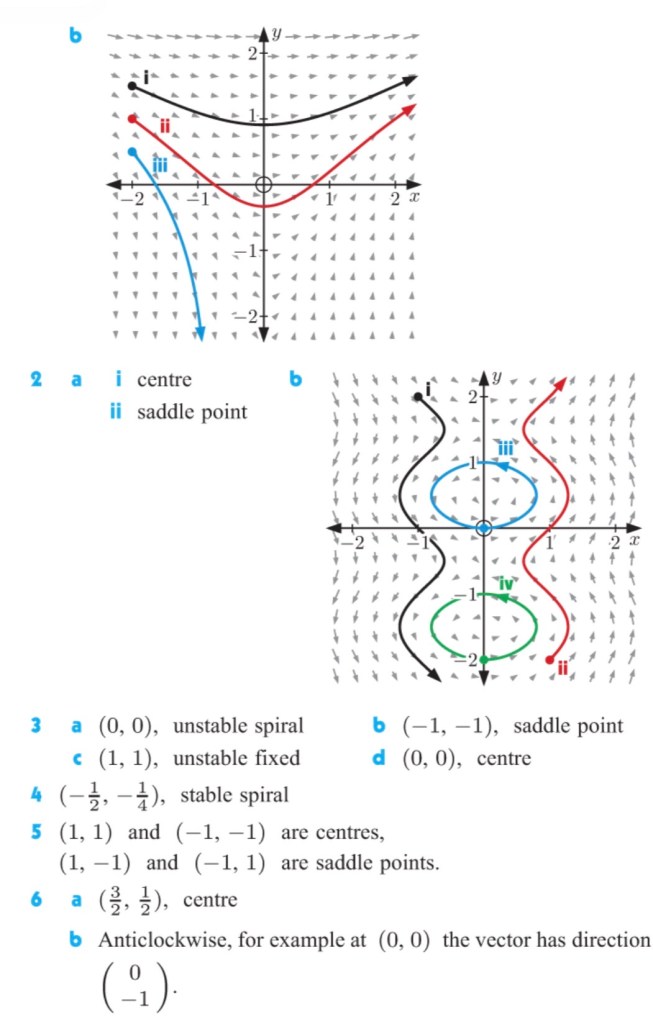
2. The phase portrait is shown below for the coupled system of DEs:

$\dot{x} = cos \pi y$
$\dot{y} = x$

(a) Show that the following points are equilibrium points. Describe the equilibrium point in each case:
- (i) (0, $\frac{1}{2}$ )
- (ii) (0 , $\frac{3}{2}$ )
(b) Illustrate the solution curve starting at:
- (i) (-1,2)
- (ii) (1,-2)
- (iii) (0,0)
- (iv) (0,-2)

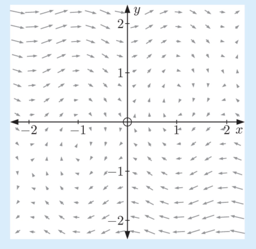
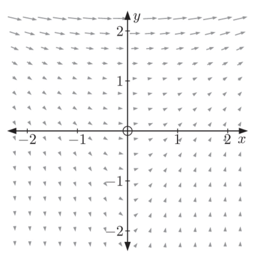
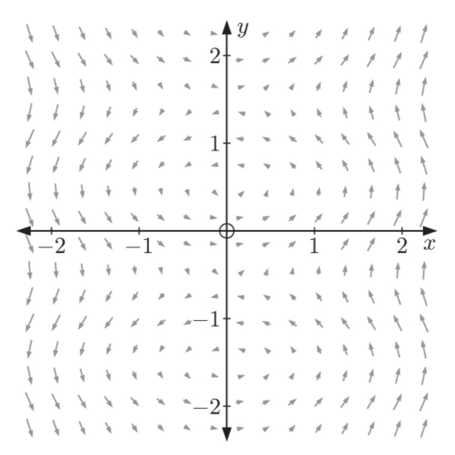
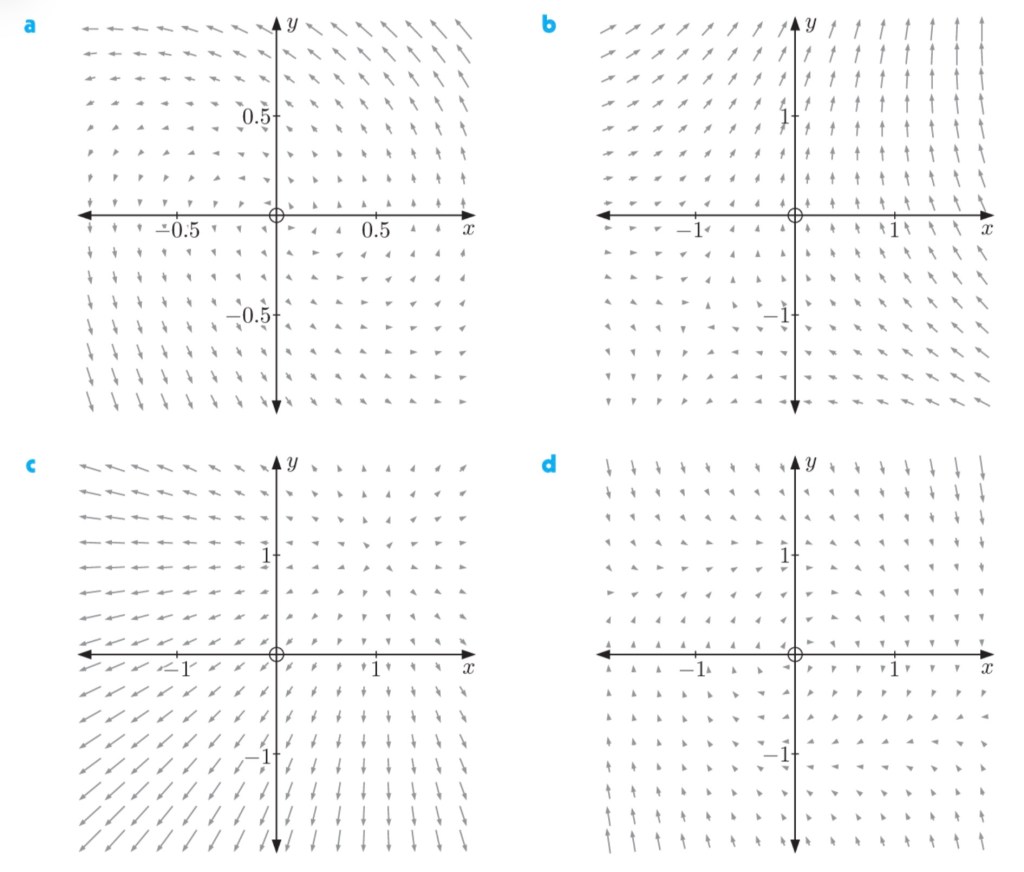
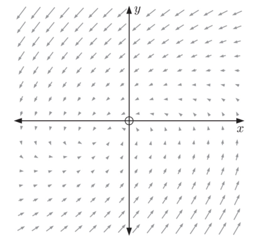
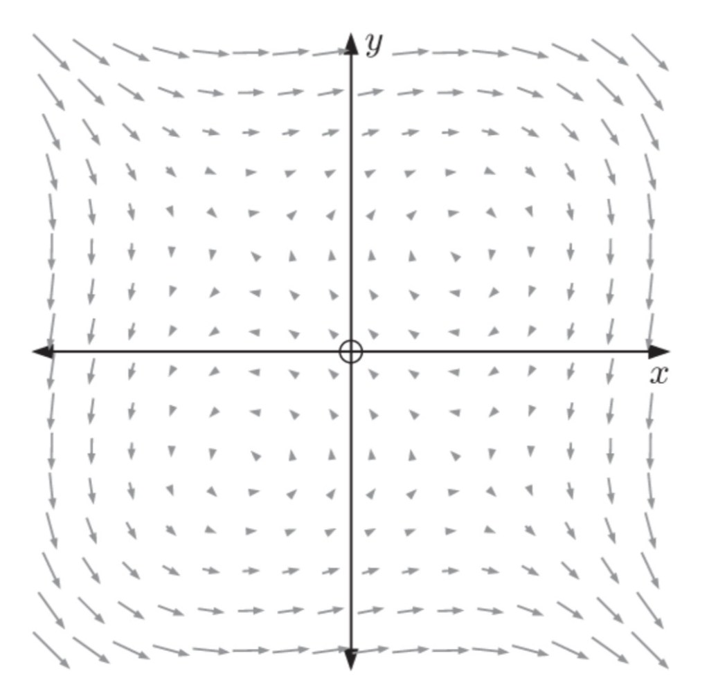
3. For each of the following phase portraits, locate and describe the equilibrium point (drawing some trajectories may help with this):

4. The diagram below shows the phase portrait for the following system of equations:

$\frac{dx}{dt} = -2y - \frac{1}{2}$
$\frac{dy}{dt} = x - 2y$ . Locate and describe the equilibrium point.

5. The diagram below shows the phase portrait for the following system of equations:

$\frac{dx}{dt} = y^2 - 1$
$\frac{dy}{dt} = 1 - x^2$ . Locate and describe the equilibrium point:

6. The diagram below shows the solution curves for the coupled system:

$\dot{x} = x - 3y$
$\dot{y} = x - y - 1$

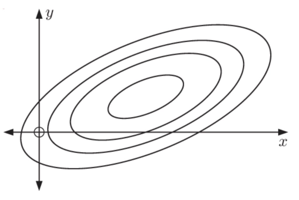
(a) Locate and describe the equilibrium point
(b) Do the solution curves rotate clockwise or anti-clockwise? Explain your answer.

Answers

IBDP. AI. HL. DEs. Phase Portraits

Share this: