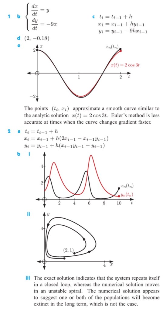
We can use Euler’s method to numerically approximate the solution to coupled equations:

, for selected initial conditions x₀ and y₀ at initial time t₀.

We choose a small time step, h>0 and then as before we calculate:

t₁ = t₀ + h

x₁ = x₀ + hf₁(x₀,y₀,t₀)

y₁ = y₀ + hf₂(x₀,y₀,t₀)

We then take the newly generated point (x₁,y₁) and generate a sequence of coordinates (x_i,y_i) for each time t_i, using:

t_i+1 = t_i + h

x_i+1 = x_i + hf₁(x_i,y_i,t_i)

y_i+1 = y_i + hf₂(x_i,y_i,t_i)

Note that the solution curve is only an approximation.

If the system has the following form:

, i.e. with derivatives independent of time, then the system is steady and we can also generate a phase portrait to study the system.

Worked Example 1

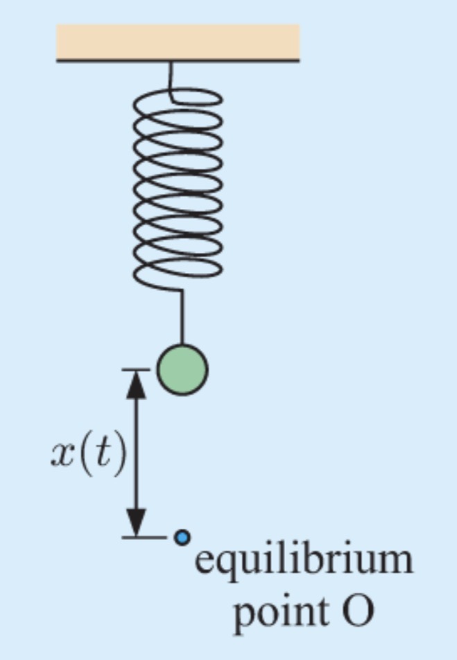
The damped simple harmonic motion of a mass on a spring is given by , where x is the displacement at time t. The mass has initial displacement 5cm and is released with velocity 0.5cms^-1 downwards.

(a.) Let be the velocity function. Hence describe the system using coupled differential equations.

(b.) Apply Euler’s method by hand with h = 0.01 to generate (x₁,y₁)

(c.) Calculate Euler’s method with h=0.01 for the first 5 seconds of motion. Plot the set of points {(t_i,x_i)} on the same set of axes as the analytic solution . Discuss your answer.

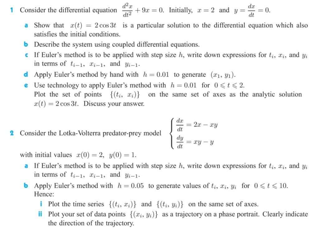
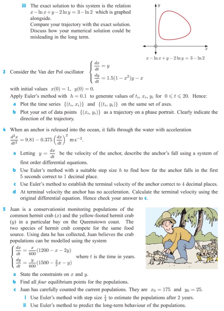
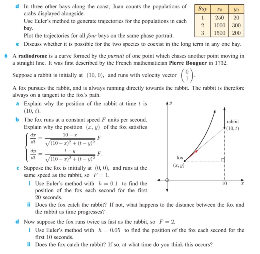
Exercise 1

Exercise 1 – Answers