Aggregate Demand

Aggregate demand is the total amount of effective demand in the economy. It comprises:

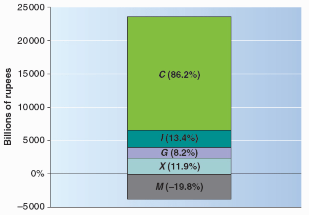
• C: Consumption: This is the largest component and is household spending on goods and services. This is mainly influenced by household’s real income;
• I: Investment: This is spending by firms, for instance on new machinery or transport equipment. Such investment enables higher production of goods in the future. It is influenced by firms’ predictions of future opportunities and the availability of funds, either internally generated, or from loans;
• G: Government Expenditure: This may be partly consumption and partly investment and is typically based on targeted needs;
• M: Imports: Purchase of goods and services that are produced elsewhere in the world (note – this is a negative amount, reducing the level of aggregate demand);
• X: Exports: Purchase by foreign consumers and firms of goods and services in the domestic economy.

The difference between exports and imports is called the trade balance.

Below, as an example, we show the components of aggregate demand in Pakistan in 2011:

An aggregate demand curve (AD) shows the relationship between the level of aggregate demand in an economy and the overall price level. It shows planned expenditure at any given overall price level.

Note that price in this context is an average of all prices of goods and services in the economy.

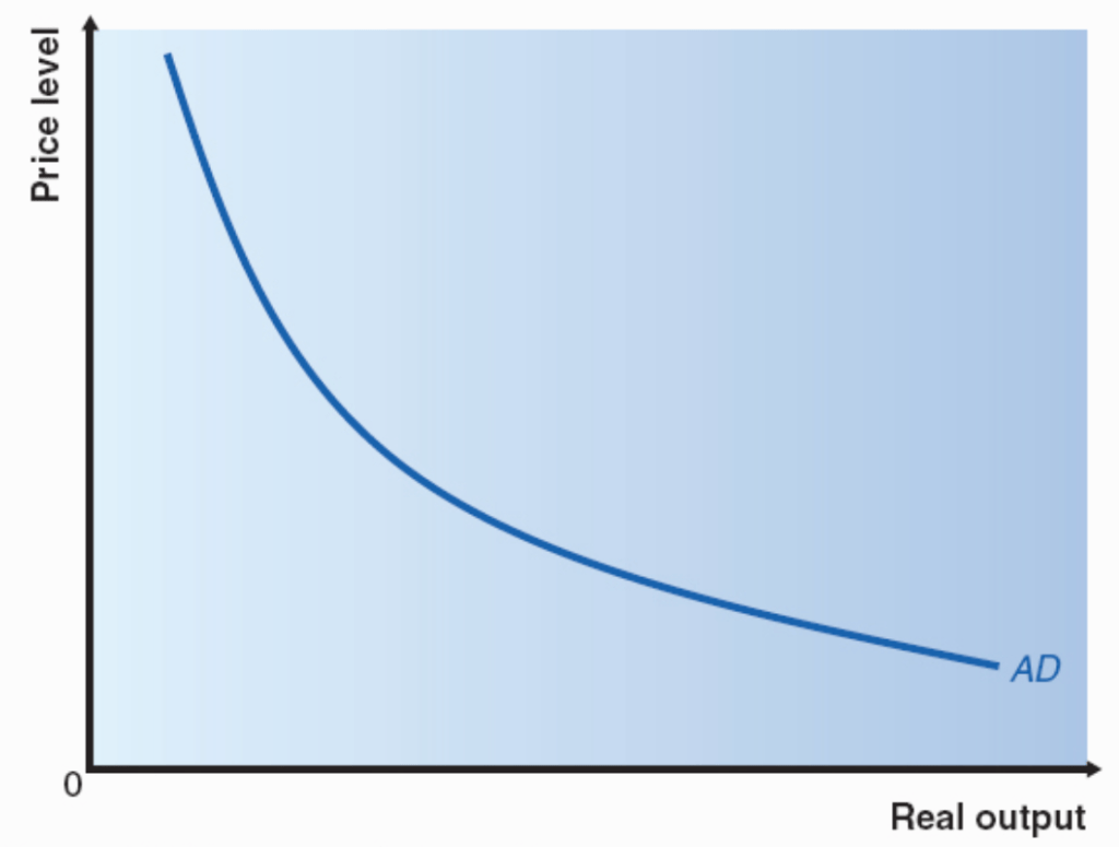
Note that when the price level is low, this means that the purchasing power of income is high, so in real terms, income is high and the real value of household’s wealth is also raised. So, ceteris paribus, a low price level leads to relatively high consumption (known as the wealth effect).

Also, when prices are low, interest rates tend to be low (due to lower demand for money), so borrowing is cheap, which also encourages consumption and investment (known as the interest rate effect).

If we consider exports and imports, low domestic prices will typically increase the competitiveness of domestically produced goods, increasing foreign demand for exports, and decreasing domestic demand for imports (known as the international effect).

Each of these arguments supports the fact that the curve is downward sloping, as a decrease in price level leads to an increase in aggregated demand.

Aggregate Supply

We can’t calculate aggregate supply simply by adding up all the individual supply curves from individual market, because an increase in price may lead to higher supply in one market as firms switch from other markets in search of higher profits. We must focus on the overall price level and the total amount supplied.

The quantity of output supplied depends upon the quantities of factors of production (labour, capital etc.) employed. It can take time to alter supply, so it is necessary to distinguish between short run aggregate supply (SRAS) where there is little flexibility, so increasing labour output, for instance, requires paying existing workers overtime, which is typically a short term measure, and long run aggregate supply (LRAS) which is influenced by the availability and effectiveness of factor inputs and improvements in technology.

Macroeconomic Equilibrium

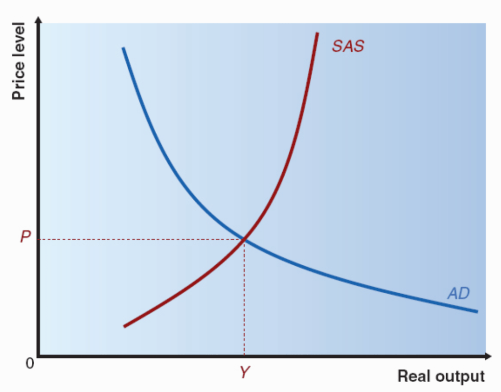
Once we have identified macroeconomic equilibrium, we can do some comparative static analysis. A shift in the aggregate demand curve can be due to any non-price level influence, e.g. changes in:

• Consumption;
• Investment;
• Government spending; or
• Net exports.

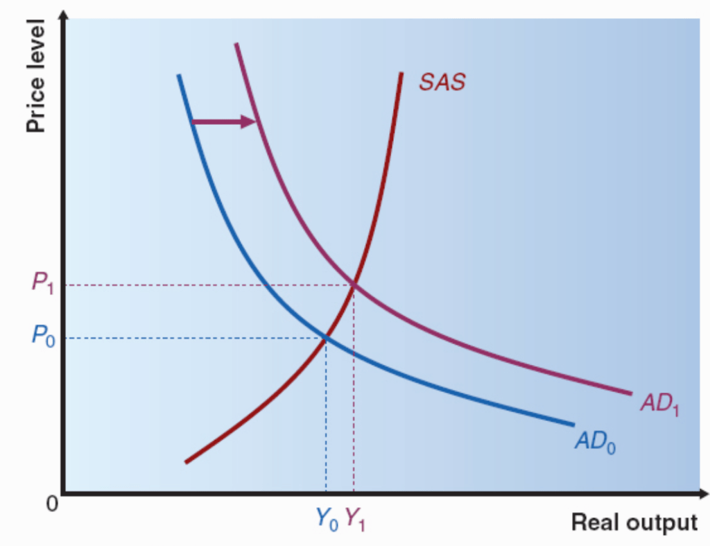
For instance, an increase in government expenditure can shift the aggregate demand curve, as shown below. However due to the increasing steepness of the supply curve, further shifts to the demand curve will lead to increases in the price level, without commensurate increases in real output (elasticity of supply reduces).

It can be argued, that the aggregate supply curve eventually becomes vertical, as there is a maximum level of output that can be produced given the factors of production available:

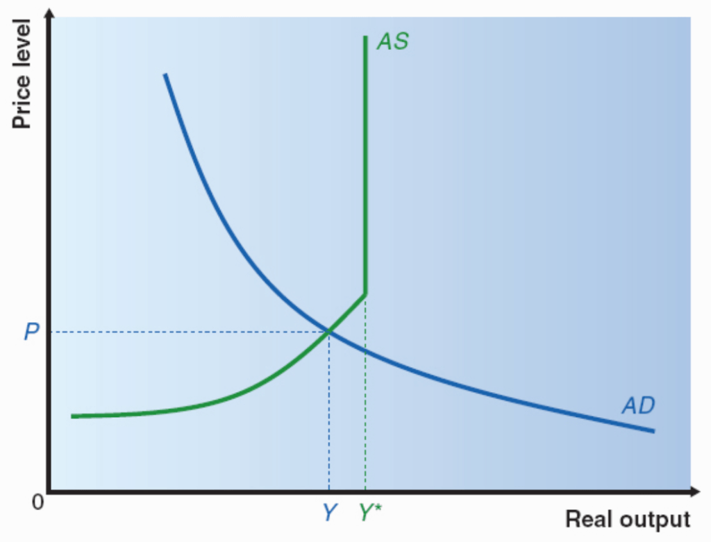
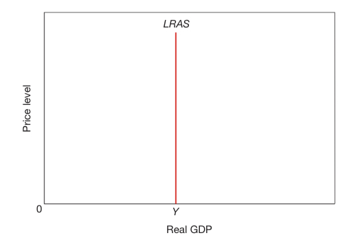
The above graph is how Keynesian Economists often represent the LRAS curve,as perfectly elastic at low rates of output, and perfectly inelastic at high rates of output, representing their view that in the long run an economy can operate at different levels of output, and not necessarily full capacity. By contrast, the New Classical Economists believe that in the long run an economy will operate at full capacity, and so represent the LRAS as a vertical line, as shown below:

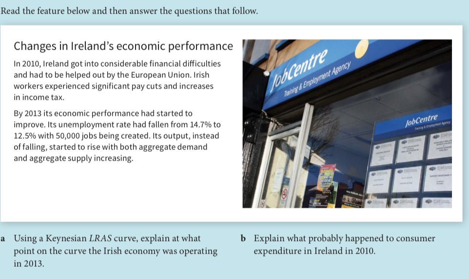
Task – LRAS

Supply shocks
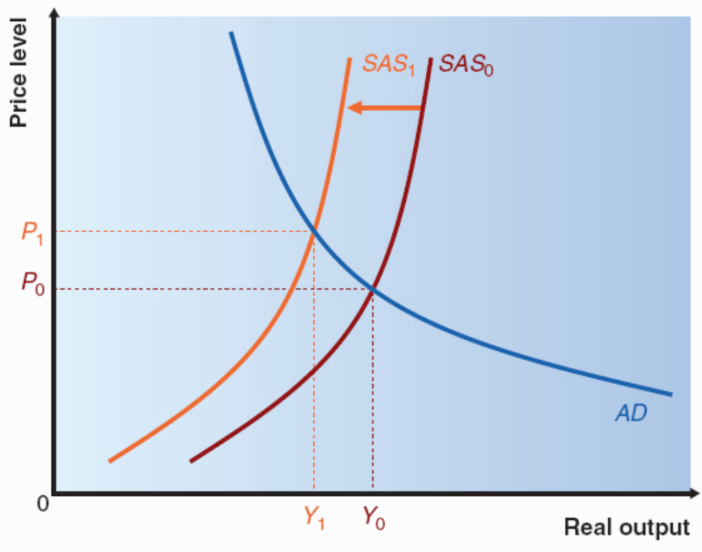
An external shock may affect aggregate supply, for instance a disaster in the Middle East could lead to an increase in oil prices, raising firms’ costs and leading to a reduction in aggregate supply, as shown below:

Movements along curves vs. movements of curves

As previously with supply and demand, we must distinguish between shifts of the AD and AS curves and shifts along them. A shift of the AS curve causes a shift along the AD curve, and vice versa. In analysing the effects of a shock, first we consider whether it affects AD or AS, then we analyse whether it is positive or negative.

The following are potential causes of a shift to the right of the LRAS:

• Net immigration;
• Increase in retirement age;
• More women entering work force;
• Net investment;
• Discovery of new resources; and
• Land reclamation (e.g. Singapore / Dubai).

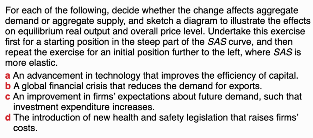
Task – Impacts on aggregate supply and demand

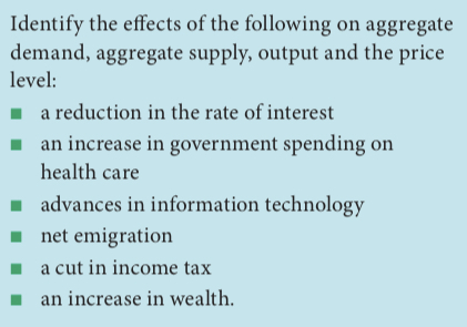
Exercise

For each of the above examples, indicate whether the result is a shift of or a movement along the AD and AS curves.