Introductory Task

Labour is one of the factors of production. It is considered a derived demand, as it is required for that output that it produces. Total physical product of labour (TPP_L) is a short-run production fuction, i.e. capital cannot be varied. Hence there are diminishing returns to labour, i.e. as labour input increases, ouput does not increase by the same amount. We can see this on the graph below, by considering the marginal physical product of labour (MPP_L), i.e. the additional quantity of output produced by an additional unit of labour input:

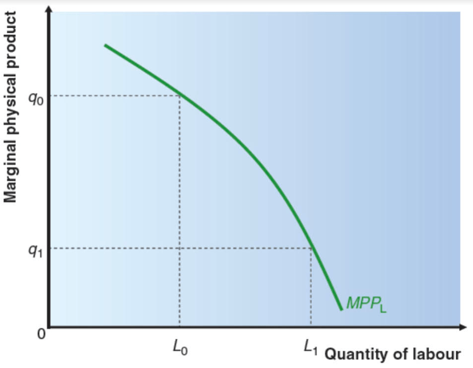
Here we see that at a relatively low level of labour input, the additional output produced by an extra unit of labour is relatively high (e.g. q₀ at L₀) but when more labour is added, the marginal physical product reduces to q₁. As the firm is interested in maximising the revenue it receives from selling the additional output, they need to consider the marginal physical product multiplied by the marginal revenue received from selling the extra output, known as the marginal revenue product of labour (MRP_L).

In a perfect competitive market, marginal revenue and price are the same, and so MRP_L is MPP_L multiplied by the price. If a firm faces a downward sloping demand curve however, it has to reduce the price of the product in order to sell additional output. Marginal revenue is then lower than price (as price must be reduced on all output sold, not just the last unit.

The below diagram considers a firm operating under perfect competition setting out to maximise profits:

Here the marginal revenue product curve is downward sloping. The ideal amount of labour input to use depends on this and on the cost of labour, which is primarily the wages paid to workers. Hence the wage (in a perfectly competitive market) can be considered as the marginal cost of labour (MC_L). Clearly, if the wage is W* above then profits are maximised when quantity of labour is at L*. This type of thinking is called marginal productivity theory.

Task – Marginal product of labour

The table below shows how the total physical product of labour varies with labour input for a firm operating in competitive product and labour markets. The price of the product is $5 and the wage rate is $30:

Labour input per period	Output (goods per period)
0	0
1	7
2	15
3	22
4	27
5	29

• Calculate the marginal physical product of labour at each level of labour input;
• Calculate the marginal revenue product of labour at each level of labour input;
• Plot the MRP_L on a graph and identify the profit-maximising level of labour input.
• Suppose that the firm faces fixed costs of $10. Calculate total revenue and total costs at each level of labour input, and check the profit-maximising levl.

Factors affecting the position of the demand for labour curve

Anything that affects the marginal physical product of labour will also affect the MRP_L. This could be an advance in technology raising labour productivity for instance. We see this below:

Demand is initially at MPR_L0, but improved technology shifts the curve to MPR_L1. If wages remain at W*, the quantity of labour hired by the firm increases from L₀ to L₁.

Also, in the long run, an expansion in a firm’s capital will also affect the demand for labour.

As MRP_L is MPP_L multiplied by marginal revenue, so changes in marginal revenue will affect labour demand. In a perfectly competitive product market, this means that changes in the price of the product will also affect labour demand. So a fall in demand for the product will mean the equilibrium price falls, which will have a subsequent effect on the firm’s demand for labour, as illustrated below:

Initially L₀ labour was demanded at wage W*, but the fall in demand led to a fall in marginal revenue product (despite no change in physical productivity of labour). So only L₁ labour is now demanded at wage rate W*. This reminds us that demand for labour is a derived demand and is tied to demand for the firm’s product.

Elasticity of Demand for Labour

When we studied PED, we noticed that the most important influences on PED were:

• availability of substitutes;
• relative size of expenditure on good within overall budget; and
• time period.

Similar influences apply when looking at elasticity of demand for labour:

• Regarding substitutes, we consider the extent to which other factors of production, such as capital, can be substituted for labour. If they can be easily substituted then, ceteris paribus, an increase in wage rate will cause the firm to more significantly reduce its demand for labour.
• Regarding relative size of expenditure, in most service industries, labour is a highly significant share of costs, so firms are very sensitive to changes in the cost of labour, whereas in capital-intensive manufacturing activity, labour may comprise a much smaller share of total production costs.
• Regarding time period, the longer term gives firms an opportunity to adjust factors of production to a different balance, investing in capital that reduces the dependence on labour.

There is an additional influence on demand for labour, because it is a derived demand, which is the PED of the product. The greater the PED of the product, the more sensitive the firm will be to a change in the wage rate, as the higher PED reduces the possibilities of passing these extra costs on to the consumer (in the form of higher prices).

Task

Using diagrams, explain how each of the following will affect a firm’s demand for labour:

• A drop in the selling price of the firm’s product;
• Adoption of working practices that improve labour productivity;
• An increase in the wage (i.e. where the firm must accept the wage as determined by the market);
• An increase in demand for the firm’s product.

Labour Supply

Previously we have considered labour supply from the perspective of a firm in a perfectly competitive market, so that the firm sees the labour suppy curve as completely elastic.

For the industry as a whole however, labour supply isn’t likely to be flat. Intuitively it should be upward-sloping, as at a higher wage more people will become available for work. There are further complexities though.

Consider an individual worker deciding how many hours of labour to supply. Each choice has an opportunity cost, so taking more leisure time involves missing out on earning oppotunities, i.e. the wage rate is the opportunity cost of leisure. So if the wage rate increases, it has two effects, which each work in opposite directions:

• SUBSTITUTION EFFECT: Leisure time is more costly so workers are motivated to work longer hours); and
• REAL INCOME EFFECT: Worker now has a higher level of real income, so they are incentivised to consumer more goods and services, including leisure.

We could argue that at relatively low wages the substitution effect will be the dominant one but that tas wage rises the real income effect will prevail. The individual labour supply curve will then be backward bending, as illustrated below:

There are other factors that influence labour supply, such as job satisfaction (which may induce a worker to accept a lower wage) and other non-pecuniary benefits, such as social facilities, training opportunities, job security, or a subsidised staff canteen.

At the industry level, the labour supply curve can be expected to be upward sloping, as although the individual workers have backward bending curves, when taken in aggregate, higher wages will induce people to join the market, either from outside the previous work force, or from industries where wages have not risen.

Labour market equilibrium

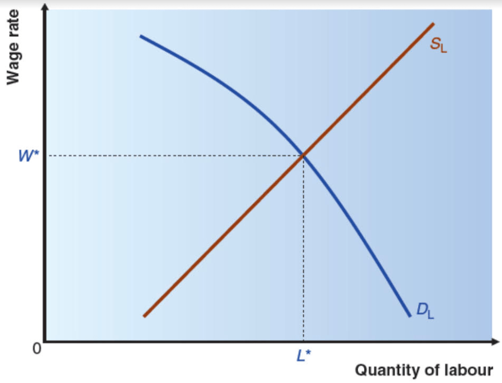
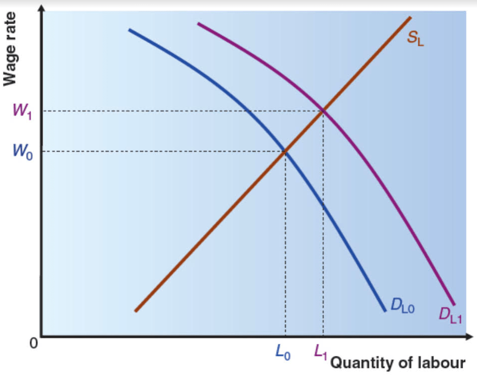
Above we see a downward sloping labour demand curve based on marginal productivity theory, and an upward sloping labour supply curve. If wage is lower than the equilibrium wage of W* then employers will not be able to fill their vacancies and will need to offer a higher wage to attract more workers. If it is higher than W*, there will be an excess supply of labour and so firms will start to reduce the wages offered until it returns to equilibrium. We can use comparative static analysis to consider changes in the labour market, for instance an increase in demand for the firm’s product will shift the demand curve to the right, as shown below:

Labour markets

There is no single labour market in an economy, just as there is no single market for goods.

Many factors of production have some flexibility, i.e. they can be used for alternative purposes. There is an opportunity cost of using a factor of production for one particular job. For instance, a woman may work in a cafe because the pay is better than she could earn working in a shop. The opportunity cost is the pay she would have earned in the shop. If the shop raises its rate of pay, there will come a point when the opportunity cost of working in the cafe has become too high and so she may decide to work in the shop. The point at which is there is referred to as transfer earnings, i.e. the minimum payment required to keep a factor of production in its present use. Any surplus wage paid beyond this is known as economic rent.

The above diagram illustrates transfer earnings and economic rent. At the equilibrium wage rate, W*, a worker is supplying labour at the margin and that worker would leave the labour market if the wage rate dropped at all. So the wage rate is the transfer earnings of that marginal worker. The same is true all along the labour supply curve. The economic rent can be seen on the graph as the additional amounts paid to workers beyond what they would accept in order to retain the “most demanding” marginal worker.

In balancing transfer earnings and economic rent, the elasticity of labour supply is very important. Compare the two extreme situations shown below, perfectly elastic labour supply and then perfectly inelastic labour supply.

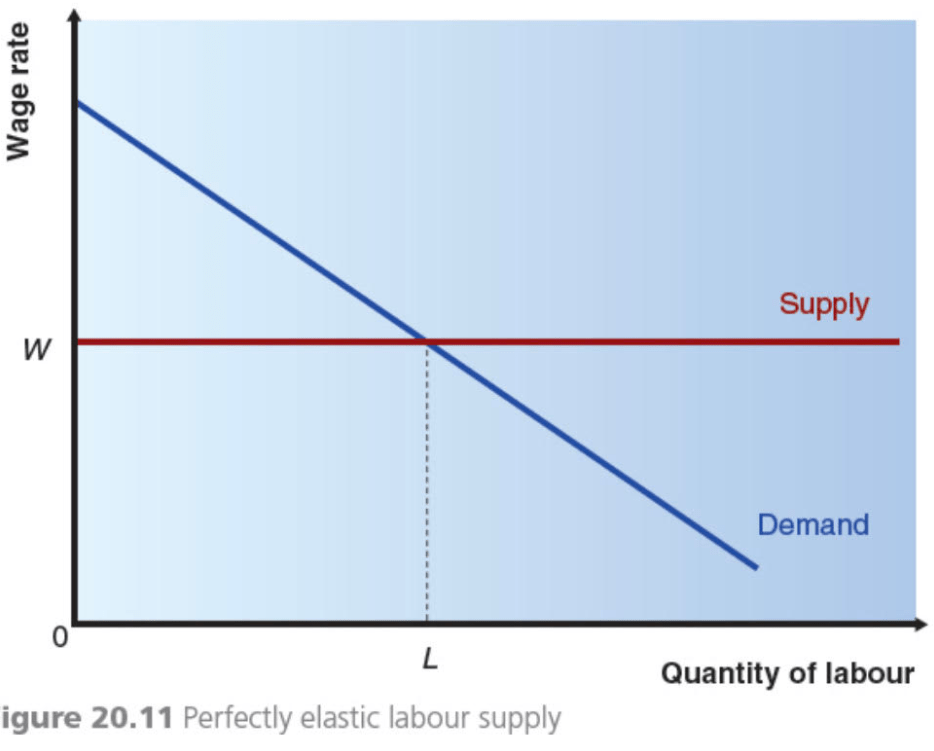
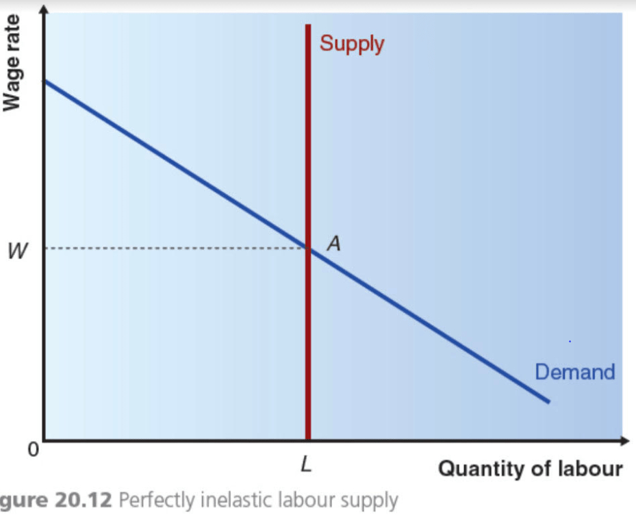
With perfectly elastic labour supply, there is a limitless supply of labour at wage rate R, so all earnings are transfer earnings, i.e. there is no economic rent. If wage is reduced below W, all workers will leave the market. With perfectly inelastic labour supply, there is a fixed amount of labour being supplied to the market, and any change in the wage rate will not affect this amount of labour. The entire earnings of the factor are now comprised of economic rent. So, in general, the more inelastic supply is, the greater proportion of total earnings that will be made up of economic rent.

In practice, more specialist jobs (e.g. heart surgeons) have a relatively inelastic supply, particularly in the short run. Hence their salary is largely composed of economic rent. This is compounded by the fact that once trained as a heart surgeon, people’s willingness to exit the market and work as a shop assistant, for instance, is reduced.

We have considered the supply side of the market, but demand is also important. It is the high demand for talented football players that increases their equilibrium wage (in addition the the inelasticity of supply).

Education and the labour market

We can think of education as a barrier to entry into a labour market that affects the elasticity of labour supply. Economists expect that in the long-run there exists an equilibrium level of wage differential, based on preferences an natural talents. These equilibriums change over time however, e.g. when computers became widely available demand rose for computer programmers as few people had this capacity. as a result many training courses and education opportunities became available, eventually leading to this wage differential reducing. This is an example of the market system working effectively to allocate resources.

Consider individuals deciding which education course to take. This is an example of cost-benefit analysis. However costs tend to come in the short-run whereas benefits come in the long-run.

Task

Imagine that you are considering whether or not to go to university. List the benefits and the costs that you expect to encounter if you choose to go. Discuss how you would balance these costs and benefits, remembering that the timings need to be taken into account.

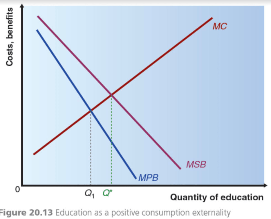
Regarding externalities (in the case of education the benefits to society of individuals being better able to cooperate and work together), the below graph shows that if the marginal social benefit is higher than the marginal private benefit then individuals tent to demand too little education (i.e. Q₁ instead of Q*):

Market Failure in Labour Markets

Market failure can occur on either the demand side or the supply side of the labour market:

• Demand side: Employers (i.e. the consumers of labour) may have market power that can be exploited at the expense of workers. Employers may act against the interests of certain groups of workers due to discrimination in their hiring practices or wage setting;
• Supply side: Supply of some types of labour may be restricted. Trade unions may be able to bid wages up to a level above the free-market equilibrium.
• We can also consider unemployment as an indication of disequilibrium in the labour market. Certain government interventions may also have unintended effects on labour markets.

A market where there is a single buyer of a good, service or factor of production is called a monopsony. A monopsonist doesn’t have to accept the equilibrium wage due to the intersection of demand and supply, but faces the market supply curve of labour directly. The supply curve is its average cost of labour, as it shows the average wage rate it must offer to obtain a specific quantity of labour input.

Below we see the monopsonist’s demand curve for labour, which is the marginal revenue product curve (MRP_L) and its supply curve of labour (AC_L):

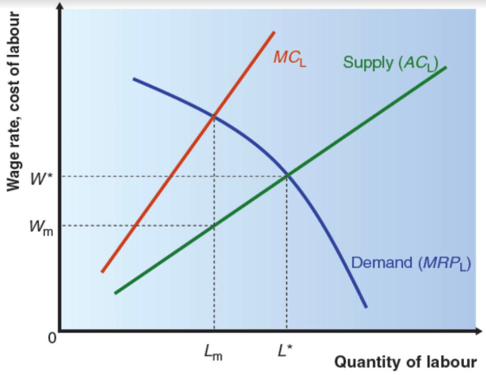
For a monopsonist to hire more labour, they must offer a higher wage to encourage more workers to join the market. This wage must then be paid to all workers, so the marginal cost of hiring an extra worker includes the increased wage to all workers. So we are able to add the marginal cost of labour curve (MC_L) to the diagram. To maximise profit, a monopsonist should hire labour up to the point where the the marginal cost of labour equals the marginal revenue product of labour (i.e. L_m). To entice sufficient workers they must pay wage W_m. Hence we see that a profit-maximising monopsonist uses less labour and pays a lower wage than a firm operating under competitive conditions. This represents a cost to society.

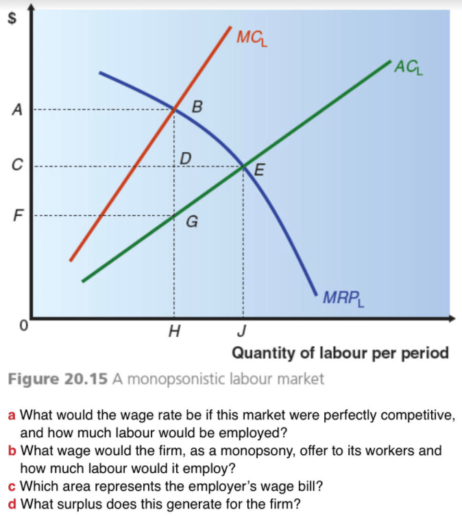
Task

Government Intervention

Unemployment is often considered a key indicator of an economy’s performance and an important cause of poverty. In recent years many societies have focused on health and safety at work and ensuring that employees are not exploited. Hence it is an important issue for governments, that have introduced various measures to try and regulate labour markets. These measures don’t always have their intended effects.

Minimum Wage

A government mandated minimum wage seeks to achieve three objectives:

• Protect employees from exploitation;
• Improve work incentives to avoid the problem of voluntary unemployment; and
• Alleviate poverty by increasing the standards of society’s poorest groups.

Critics suggest that none of these objectives are achieved, as firms can always work around the minimum wage to continue to exploit employees (e.g. by paying a piecework rate so there is no set hourly wage), and such policies are considered as lacking sufficient focus to tackle poverty. Most importantly though, a minimum wage is seen as causing an increase in unemployment because of its effects on labour demand.

The below graph considers a firm operating under conditions of perfect competition (so they must accept the wage set by the market):

If a firm’s demand curve is represented by its marginal revenue product curve, MRP_L, then in a free market it must accept the equilibrium wage W* and so uses labour l*. A government minimum wage will reduce labour to d_min, as it is not profitable to employ labour beyond this point.

The result is similar for all other firms in the market. Below we see the combined result on the market (where the supply curve of labour is upward sloping, as it is the market supply curve). Here the free-market equilibrium demand is L* and the equilibrium wage rate is W*:

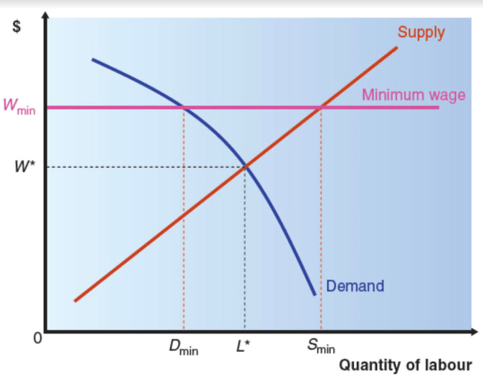
If the government sets the minimum wage at W_min, all firms reduced their demand for labour at the higher wage. Combined demand is now D_min, but avaialable labour supply is now S_min. The difference between these is unemployment. Note that the unemployment is due to two reasons, lower demand at the higher wage rate and higher supply at the higher wage rate.

If the minimum wage is set below the equilibrium level, it will have no impact. Also, if a labour market has a monopsony buyer of labour, as shown below, the firm sets its marginal cost of labour equal to its marginal product, offering a wage of W₀ and hiring L₀ labour:

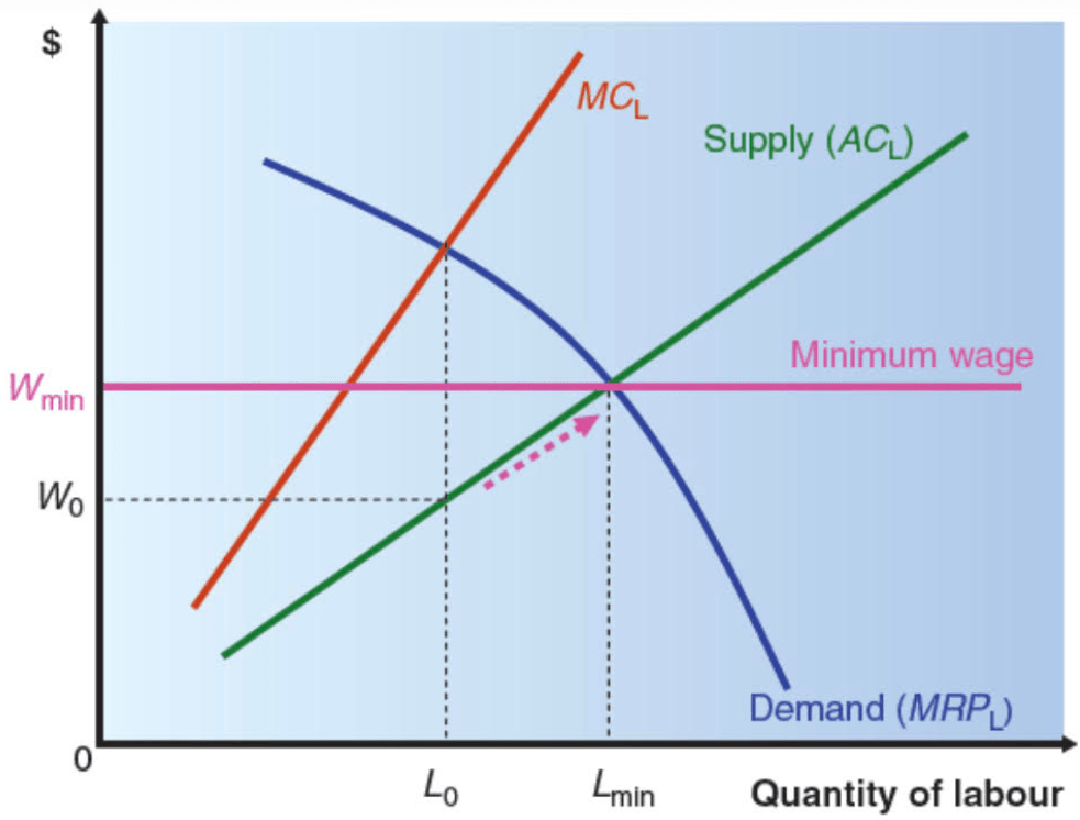
A minimum wage W_min, will mean that the firm hires labour up to the point where the wage is equal to the marginal revenue product, which brings the market back to the position it was in under perfect competition.

It is very difficult for the government to gather sufficient information to set a minimum wage at exactly the right level to produce this outcome. Nevertheless, any wage between W₀ and W_min will encourage the firm to increase its employment. If the minimum wage goes above the competitive equilibrium level, again it will lead to some unemployment.

Task – Living Wage

Trade unions

A trade union is an organisation of workers that negotiates with employers on behalf of its members. Their three major objectives are:

• Wage bargaining;
• Improved work conditions; and
• Security of employment for members.

They can affect labour market equilibrium by limiting the supply of workers in an industry, or by successfully negotiating for higher wages for their members. Both have similar effects on equilibrium.

The graph below considers the impact of restricting labour supply (for a firm with a demand curve based on marginal productivity theory):

W* is the average going wage in the economy, at which wage the firm is prepared to employ labour up to L₀. If a trade union restricts labour to L₁, then the firm will be able to increase the wage to W₁. This may benefit a “closed shop” union, that ensures that a firm only employs members of the union. Effectively the union is trading off higher wages for its members in exchange for a lower level of overall employment. The extent of the trade off depends on the elasticity of demand for labour, as illustrated below, where relatively elastic demand is shown by demand curve D_L0 and relatively inelastic demand is shown be demand curve D_L1.

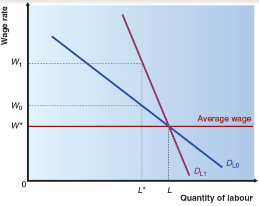
This is intutively logical, as there will be low elasticity of demand in situations where (1) firms cannot readily substitute capital for labour, (2) labour forms a small part of overall costs, and (3) PED of the firm’s product is relatviely inelastic. (1) gives the union a relatively strong bargaining position, (2) makes the firm likely to allow a wage increase as its effect will be limited, and (3) means the firm may be able to pass the wage increase on to the customers.

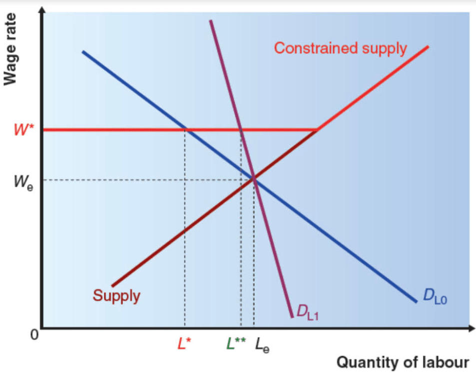
The primary function of a union is to negotiate higher wages for its members, as illustrated below:

In the absence of a union, the equilibrium, where demand and supply intersect, causes the firm to hire L_e of labour at a wage of W_e. If a trade union negotiates a wage of W*, the supply curve is altered (as shown by the pale red line). The firm now employs only L* labour at this wage. So, as before, a greater wage is acheived at the expense of greater unemployment. Again, elasticity of demand effects the outcome, as illustrated below:

The involvement of a trade union can give workers more job security, as the union protects their interests. From a firm’s perspective this may be positive as it may lead to workers being more productive, or more willing to accept changes in working practices that increase productivity.

A further criticism of trade unions is that they have reduced the degree of flexibility of the labour market, primarily by limiting the entry of workers into a market.

Closing Task