Introductory Task

Open and Closed Economies

An economy that engages in international trade is called an open economy, whereas one that doesn’t export or import goods and services is called a closed economy (this is a theoretical concept, because in practice no economy is completely closed).

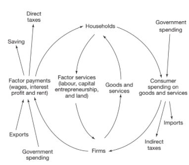
The circular flow of income shows how income and spending move around an economy, shown below for a closed economy. The inner circle shows the real flow of products and factor services and the outer circle the money flow of spending and incomes:

In practice, there is some leakage from the circular flow, as some income is saved, some is taxed and some is spent on imports. There are also additional injections, due to foreign investment and foreign spending on domestic products. The below diagram, for an open economy, includes these:

Multiplier (also known as National Income Multiplier or Keynesian Multiplier)

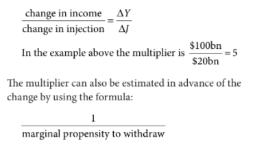
The multiplier shows the relationship between an initial change in spending and the final rise in GDP. It occurs because a rise in expenditure creates incomes, some of which are then spent creating further incomes. e.g. If people spend 80% of any extra income, an increase in government spending of $20b will cause a final rise in GDP of $100b. (e.g. because $20b spent by the government will lead people to spend $16b of their extra incomes, which will lead to a further group of people spending $12.8b, etc. until incomes have increased to $100b and the change in injections is matched by the change in withdrawals).

The multiplier is calculated after the injections as follows:

Multiplier and equilibrium income in 2-, 3- and 4-sector economic models

Economists typically start by analysing a simplified model and then gradually add more variables to the model. With the multiplier, we start by considering an economy with only 2 sectors, then consider one with 3 sectors and then one with 4.

A two-sector economy includes households and firms. Here there is only one withdrawal (saving, “S”) and one injection (investment, “I”). In such an economy, if “mps” means “marginal propensity to save” (i.e. the proportion of extra income which is saved), the multiplier is , or or alternatively . This is because in this model income is either spent or saved. Equilibrium income occurs where aggregate expenditure equals output (i.e. C + I = Y )and injections equal withdrawals (i.e. I = S). This is sometimes referred to as “a closed economy without a government sector”.

A three-sector economy also includes the government. This gives an extra injection (government spending, “G”) and an extra withdrawal (taxation, “T”). The multiplier becomes . mrt is marginal rate of taxation, which is the proportion of extra income that is taxed. Equilibrium income is achieved when aggregate expenditure equals output (C+I+G=Y) and injections equal withdrawals (I+G=S+T).

A four-sector economy also includes the foreign trade sector and is an open economy. The multiplier now is where mpm is marginal propensity to import (i.e. proportion of extra income spent on imports). Now equilibrium income is where aggregate expenditure equals output, now C + I + G + (X-M) = Y and injections equal withdrawals, so I+G+X = S+T+M)

Task

In an economy, the mps is 0.1 and the mpm is 0.2. GDP is is $300b. The government raises its spending by $66b in a bid to close a deflationary gap of $20b. Calculate:

a) The value of the multiplier;

b) The increase in GDP;

c) Whether the injection of extra government spending is sufficient, too high or too low to close the deflationary gap.

Aggregate Expenditure

Aggregate expenditure is the total amount spent in the economy at different levels of GDP. It includes:

• C: Consumption;
• I: Investment;
• G: Government spending; and
• X-M: Net exports (i.e. exports minus imports).

Whereas aggregate demand curve plots total spending against different price levels, aggregate expenditure curve plots total spending against different income levels.

Consumption

This is spending by households on goods and services to satisfy their current wants. It is mostly influenced by the level of disposable income (income plus benefits minus direct taxes). As income rises, spending typically rises, but the proportion of disposable income that is spent typically falls. This proportion is called the average propensity to consume (“apc”)

With poor individuals (or countries), consumption can exceed income, if they rely on past savings or borrowing. This is called dissaving. Saving is defined as income minus consumption and the average propensity to save, aps measures the proportion of income saved and is calculated as 1 – apc. As income increases, both the total amount saved and aps increase.

The rich also have a lower marginal propensity to consume (mpc) and a higher marginal propensity to save (mps) than the poor.

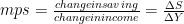
Similarly marginal propensity to save, mps = 1 – mpc. This can also be calculated by:

We can also investigate the relationship between consumption and income using the consumption and saving functions.

The consumption function, C = a+bY shows how much will be spent at different levels of income. C is consumption, a is autonomous consumption (i.e. a fixed amount spent at all levels of income, including when income is zero), b is the marginal propensity to consume and Y is disposable income. We can also define bY as income-induced consumption, because it is spending that is dependent on income.

With the saving function, S = -a+sY, S is saving, s is marginal propensity to save, Y is income and a is autonomous dissaving (i.e. how much of their savings people draw on when their income is zero (unchanged for greater levels of income)). sY is income-induced saving, i.e. saving that is dependent on income. The saving function can be used to work out how much and what proportion households will save at different income levels.

Several factors, other than disposable income, also influence consumption. These include:

• Distribution of income – If income is more evenly distributed, e.g. due to an increase in direct tax rates and state benefits, consumption typically rises;
• Rate of interest – Low interest rates generally stimulate spending (by reducing the return from savings and making credit more cheaply available);
• Availability of credit;
• Expectations – If people are optimistic that their future jobs are secure and their incomes will rise, they are likely to increase their spending.
• Wealth – Increased wealth, e.g. due to rise in house or equity prices, usually leads to increased consumption.

Investment

Investment is spending by firms on capital goods, such as factories and machinery. Influences on level of investment include:

• Consumer demand – as this increases, firms will typically need to buy more capital equipment to expand their capacity.;
• Rate of interest – A drop in the interest rate is likely to stimulate a rise in investment (as cost of investment falls – also consumer demand increases);
• Technology;
• Cost of capital goods;
• Expectations – Again, optimism about economic conditions and consumer demand will encourage increased investment; and
• Government policy – Cutting corporation tax and providing investment subsidies can increase private sector investment.

Government spending

Government spending is influenced by government policy, tax revenue and demographic changes. A government that wants to raise economic activity may choose to increase its spending, funded either by increased taxation, or by borrowing. An increase in the non-working population in society (i.e. children or elderly people) may put pressure on the government to increase spending.

Net exports

A country’s net exports is influenced by:

• The country’s GDP – If this increases, demand for imports usually increases. Some products may also be diverted from the export market to the domestic market;
• Other countries’ GDP – a rise in incomes overseas can lead to an increase in the demand for domestic exports;
• Relative price and quality competitiveness of country’s products; and
• Exchange rate – A fall in the exchange rate will make the country’s exports cheaper and imports more expensive. So if demand for exports and imports is elastic, export revenue will rise and import expenditure will fall, causing a rise in net exports.

Income Determination

Income in an economy is determined where aggregate expenditure equals current output, as per the diagram below (known as the Keynesian 45 degree diagram). (The A level textbooks don’t do it, but I find it very helpful to think of the green line here as Production and the red line as Demand).

If aggregate expenditure exceeds current output, firms will seek to produce more, they will employ more factors of production and GDP will rise, whereas if aggregate expenditure is below current output, firms will reduce production. If aggregate expenditure rises (perhaps due to an increase in consumption and investment because of increased optimism), output will increase, as shown below:

For income to remain the same, it is necessary that any injections into the circular flow of income are matched by withdrawals. If injections exceed withdrawals then there will be extra spending in the economy, causing aa rise in income. The diagrams below show firstly equilibrium in a 2-sector economy and then a rise in investment causing a rise in GDP:

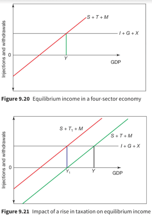
A fall in savings has a similar effect. The below diagrams shows equilibrium income where I + G + X = S + T + M in a four sector economy followed by the impact if tax rates rise without any change in government spending:

A rise in savings also causes GDP to fall. In fact a decision by households to save more can actually result in them saving less, because higher saving reduces income and hence the ability of households to save, known as the paradox of thrift.

Inflationary and Deflationary Gaps

An economy may not achieve full employment in the short run (Keynesians would argue nor in the long run). If aggregate expenditure exceeds the potential output of the economy, then there is an inflationary gap. In this case not all demand can be met, due to insufficient resources. So excess demand pushes the price level up.

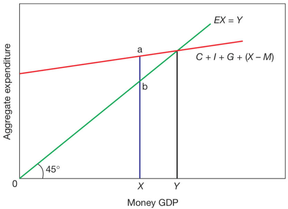
Below we see an economy in equilibrium with a GDP of Y above the level of output X that could be achieved with resources fully employed. Here ab represents the inflationary gap:

A government might use government spending or increased taxation to reduce aggregate expenditure and try to reduce the inflationary gap, as shown below:

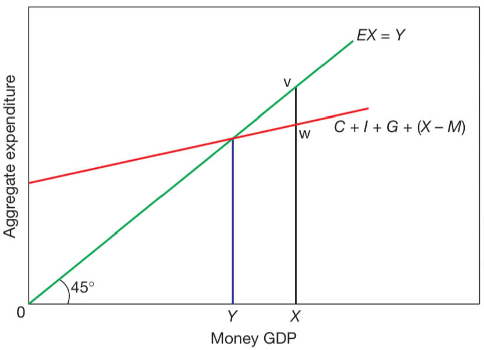
If the equilibrium level of GDP is below the full employment level, then there is a deflationary gap, as shown below, where the lack of aggregate expenditure results in an equilibrium level Y of GDP, below the full employment level of X. The deflationary gap is vw.

The Keynesian solution to a deflationary gap is to increase government spending by borrowing, as shown below:

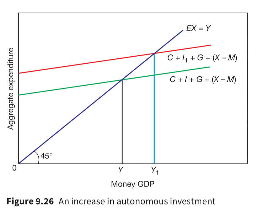
Autonomous and Induced Investment

The portion of investment that does not depend on changes of income is called autonomous investment. This might be a firm buying capital goods because they are optimistic about the future or because of a drop in the interest rate. The impact of an increase in autonomous expenditure is shown below:

By contrast, induced investment, is investment influenced by change in income, and is represented by movement along the expenditure line.

Task: Increase in Consumption

The accelerator

The accelerator theory is an economic model that suggests that investment depends on the rate of change in income and that a change in GDP will cause a greater proportionate change in investment. If a $1m increase in GDP causes induced investment to rise by $3m, the accelerator coefficient is 3.

Under this theory, if GDP rises at a constant rate, induced investment will not change, because firms continue to buy the same number of machines each year to expand capacity. However, a change in the rate of growth of income can significantly influence investment.

Consider the data below. Note that this shows a capital-output ratio of 100.

During the first year demand for consumer goods increases by 25% and then in the second year demand for capital goods increases by 200%. In the fourth year the rate of growth of demand slows and so in the fifth year demand for capital goods falls, with investment of zero, meaning that worn-out machines are not replaced and production capacity is reduced. Note that if firms have spare capacity, or expect increases in consumer demand to be temporary, then an increase in demand for consumer goods will not always lead to a greater percentage change in demand for capital goods (capital goods may also have limited availability, or be less required due to improvements in technology).

Closing Task