We are going to look at finding probability generating functions, PGFs, of discrete probability distributions, which can give us an efficient way to find expected values and variance, as well as allowing for greater analysis.
Let X represent a discrete random variable, which can take values xi for i from 1 to n, with probabilities as per the following table:
| x | x1 | x2 | x3 | … | xn |
| P(X=x) | P(X=x1) | P(X=x2) | P(X=x3) | … | P(X=xn) |
Using the table we can form the following function:
GX(t) = P(X=x1)tx1 + P(X=x2)tx2 + P(X=x3)tx3 + … P(X=xn)txn, which can be more concisely written as GX(t) = ΣtxiP(X=xi) (known as the closed form of this PGF).
Notice that GX(t) is also the same as the expectation function for tx, so E(tx) = GX(t) = ΣtxiP(X=xi).
The t we are using is effectively a dummy variable that is useful for us.
Worked Example. PGF
Consider the following probability distribution:
| x | 0 | 1 | 2 | 3 | 4 | 5 | 6 |
| P(X = x) | 0.1 | 0.2 | 0.3 | 0.15 | 0.1 | 0.1 | 0.05 |
Write down the PGF for the random variable X.
Worked Example. PGF 2
Consider the following probability distribution:
| x | 2 | 4 | 5 | 10 |
| P(X = x) | 0.1 | 0.2 | 0.3 | 0.4 |
Write down the PGF for the random variable X.
You probably noticed in the above examples that the probabilities are simply the coefficients of the t terms. Hence these coefficients sum to 1. So GX(1) = 1.
If we differentiate the PGF with respect to t, we will cause each term to be multiplied by the value xi, giving G’X(t) = Σxi(t)xi-1P(X=xi).
So G’X(1) = Σxi(1)xi-1P(X=xi) = ΣxiP(X=xi), which is the same as E(X). Hence G’X(1) = E(X).
Worked Example. PGF 3
Let X be a discrete random variable, as showing in the probability distribution given by:
| x | 1 | 2 | 3 | 4 | 5 |
| P(X = x) | 0.2 | 0.2 | 0.2 | 0.2 | 0.2 |
Find the probability generating function for X.
Standard discrete distributions
Discrete uniform distribution: If X is a discrete random variable, with a uniform distribution, that is P(X = xi) = 1/n for i = 1,2, .., n, then
Binomial distribution: Let X ~ Bi(n,p). Then
Geometric distribution: Let X ~ Geo(p). Then

Poisson distribution: Let X ~ Po(𝞴). Then
Worked Example Binary Distribution
Let X ~ Bi(5,0.2). Find the probability generating function for X.
Worked Example Geometric Distribution
Let X ~ Geo(1/5). Find the probability generating function for X.
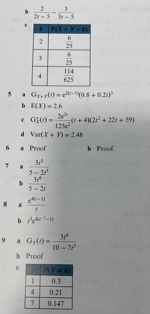
Exercise 1

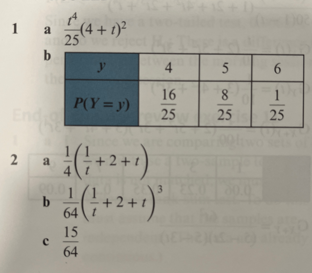
Answers to Exercise 1

Worked solutions to Exercise 1
Using the Probability Generating Function to calculate Mean and Variance
We have seen above that GX(t) = ΣtxP(X=x).
And from this it follows that G’X(t) = Σxtx-1P(X=x) and
G”X(t) = Σx(x-1)tx-2P(X=x) = Σ(x2-x)tx-2P(X=x) = Σx2tx-2P(X=x) – Σxtx-2P(X=x)
If we evaluate at t=1, we get G”X(1) = Σx2P(X=x) – ΣxtP(X=x)
So G”X(1) = E(X2) – E(X) which we rearrange to give: E(X2) = G”X(1) + G’X(1) ( as we showed above that G’X(1) = E(X).
Hence, Var(X) = E(X2) – [E(X)]2= G”X(1) + G’X(1) – [G’X(1)]2
Worked Example. Mean and Variance using PGF
A bag contains 5 red balls and 3 green balls. The balls are taken out one at a time, the colour is noted, and then it is replaced. Let X be the number of times that a ball is removed until a green ball is chosen.
(a) State the PGF of X.
(b) Calculate the mean and variance of X.
Worked Example. Mean and Variance using PGF (Poisson)
Prove that for X ~ Po(𝞴):
(a) E(X) = 𝞴
(b) Var(X) = 𝞴
Worked Example PGF
A discrete random variable has the following probability distribution:
| x | 0 | 1 | 2 |
| P(X = x) | a | b | c |
The mean is 2/3 and the variance is 5/9. Find a, b and c.
Exercise 2


Answers to Exercise 2

Worked Solutions to Exercise 2
Sum of Independent Random Variables
Statistics 2 looked at the situation where we have random variable X with Normal distribution N(μ1,𝞼12) and random variable Y with Normal distribution N(μ2,𝞼22) and we are interested in the distribution of X+Y, which is N(μ1 + μ2, 𝞼12 + 𝞼22). The same applies for the Poisson distribution.
We are now interested in finding the PGF of X+Y for independent random variables X and Y. We will consider discrete RVs.
Let us consider X, which has the following probability distribution:
| x | 0 | 1 | 2 |
| P(X=x) | p0 | p1 | p2 |
Let us also consider Y, which has the following probability distribution:
| x | 0 | 1 | 2 |
| P(X=x) | q0 | q1 | q2 |
We can hence see that the distribution of X+Y is:
| x+y | P(X+Y = x+y) |
| 0 | P (X = 0 ∩ Y = 0) |
| 1 | P (X = 0 ∩ Y = 1) + P (X = 1 ∩ Y = 0) |
| 2 | P (X = 0 ∩ Y = 2) + P (X = 1 ∩ Y = 1) + P (X = 2 ∩ Y = 0) |
| 3 | P (X = 1 ∩ Y = 2) + P (X = 2 ∩ Y = 1) |
| 4 | P (X = 2 ∩ Y = 2) |
If X and Y are independent, then P(X=xi ∩ Y=yj) = P(X=xi) x P(Y=yj) = piqj, so we can simplify the table as:
| x+y | P(X+Y = x+y) |
| 0 | p0q0 |
| 1 | p1q0 + p0q1 |
| 2 | p2q0 + p1q1 + p0q2 |
| 3 | p2q1 + p1q2 |
| 4 | p2q2 |
So we have the PGF GX+Y(t) = p0q0 +(p1q0 + p0q1)t + (p2q0 + p1q1 + p0q2)t2 + (p2q1 + p1q2)t3 +p2q2t4 which can be rewritten as GX+Y(t) = (p0 + p1t + p2t2)(q0 + q1t + q2t2), which are the PGFs of X and Y, so in fact GX+Y(t) = GX(t) x GY(t), which we call the convolution theorem.
Worked Example. Convolution Theorem
The discrete random variables X and Y have the following probability distributions:
| x | 1 | 2 | 3 |
| P(X = x) | 1/4 | 1/4 | 1/2 |
| x | 2 | 4 | 6 |
| P(Y = y) | 1/3 | 1/3 | 1/3 |
Assuming that X and Y are independent,
(a) Find the PGF of X + Y
(b) Write down the probability distribution of X + Y
(c) Show that E(X+Y) = E(X) + E(Y) and Var(X+Y) = Var(X) + Var(Y).
The PGF of a function of a random variable
Let Y = aX + b, where X has the PGF GX(t). We use the fact that GX(t) = E(tX).
So GY(t) = E(tY)
= E(taX+b)
= E(taXtb)
= tb x E(taX)
= tb x E[(ta)X]
= tb x GX(ta)
So, GaX+b(t) = tbGX(ta).
Following from this result, we have E(aX+b) = aE(X) + b and Var(aX+b) = a2Var(X)
Worked Example. Function of Random Variable
A discrete random variable X has the probability distribution:
| x | 1 | 2 | 3 | 4 | 5 |
| P(X = x) | 1/9 | 2/9 | 3/9 | 2/9 | 1/9 |
(a) Find GX(t), the PGF of X
(b) Given that Y = 4 – 7X, find GY(t), the PGF of Y.
Exercise 3


Answers to Exercise 3

Worked Solutions to Exercise 3
Three or more Random Variables
The results we have found generalise to deal with linear combinations of more than two random variables..
So, for independent random variables Xi with corresponding PGFs GXi(t),
GX1+…+Xn(t) = GX1(t) x GX2(t) x … x GXn(t).
If the n discrete random variables all have the same PGF, the formula reduces to GX1+…+Xn(t) = [GX(t)]n.
Also, GaX1 + bX2 = GX1(ta) x GX2(tb).
Worked Example. Six Random Variables
Find the PGF for the total number of 8s when a fair 8-sided dice is rolled six times.
Exercise 4


Answers to Exercise 4

Worked Solutions to Exercise 4
End of PGF Chapter Mixed Questions

Answers to End of PGF Chapter Mixed Questions

