So far all of our tests have been based on an assumed underlying distribution, for which we have been testing the parameter, e.g. the mean or the variance.
If we don’t have an assumed underlying distribution, we can use non-parametric tests. Typically with such tests the measure of location we are interested in is the median.
Below are summarised the types of non-parametric tests we will learn. Which we choose depends on whether we have a single sample or two samples and various conditions regarding the symmetry of the datasets and relationship between datasets. Note that all of the tests assume independent underlying data.
| Type of Test | Test | Assumptions |
| Single sample | SS1. Sign test | Underlying data are continuous |
| Single sample | SS2. Wilcoxon signed-rank test | Underlying data are continuous Underlying data are symmetric |
| Two samples | TS1. Paired sign test | Data are in matched pairs Differences between matched pairs are continuous |
| Two samples | TS2. Wilcoxon matched-pairs signed-rank test | Data are in matched pairs Underlying data are symmetric Differences between matched pairs are continuous |
| Two samples | TS3. Wilcoxon rank-sum test | Two samples are independent Underlying data are symmetric |
Single Sample Test 1: Sign Test
The single-sample sign test lets us identify if the median of a set of data differs from a stated median. The median is not as a a parameter, as we do not know the underlying distribution.
To perform the test, all values greater than the stated median are replaced with a “+” and all values less than the stated median are replaced with a “-“. If the data are evenly distributed about the median, we would expect a similar number of + and – signs. (N.B. Values which are neither greater nor less than the median are not included in our course, but would typically be ignored).
Effectively this is a special case of the binomial test. For n data points, we are using X ~ Bi(n, 0.5), where the test statistic is the number of + signs. We calculate the probability that X is above the test statistic, below the statistic, or, for a 2-tailed test, either above or below.
Worked Example. Single-sample sign test
The following dataset is believed to come from a population with median 135:
| 150 | 130 | 125 | 140 | 170 |
| 140 | 190 | 180 | 175 | 165 |
| 160 | 130 | 140 | 140 | 145 |
Perform a single-sample sign test at the 5% significance level to test this claim.
If n is large, we can also use the normal distribution with the sign test, as follows:
Let S = min(number of + signs, number of – signs). Then E(S) = n/2 and Var(S) = n/4.
For large n (n must be > 10), T ~ N(n/2 , n/4), we can use the normal approximation of the binomial with p = 0.5. We must also use a continuity correction (as we our using a continuous distribution to approximate a discrete distribution), so our x-value is

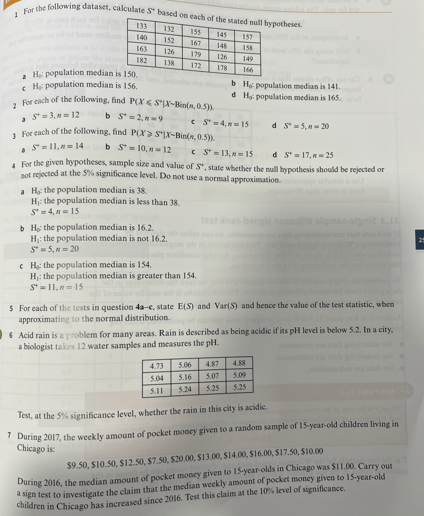
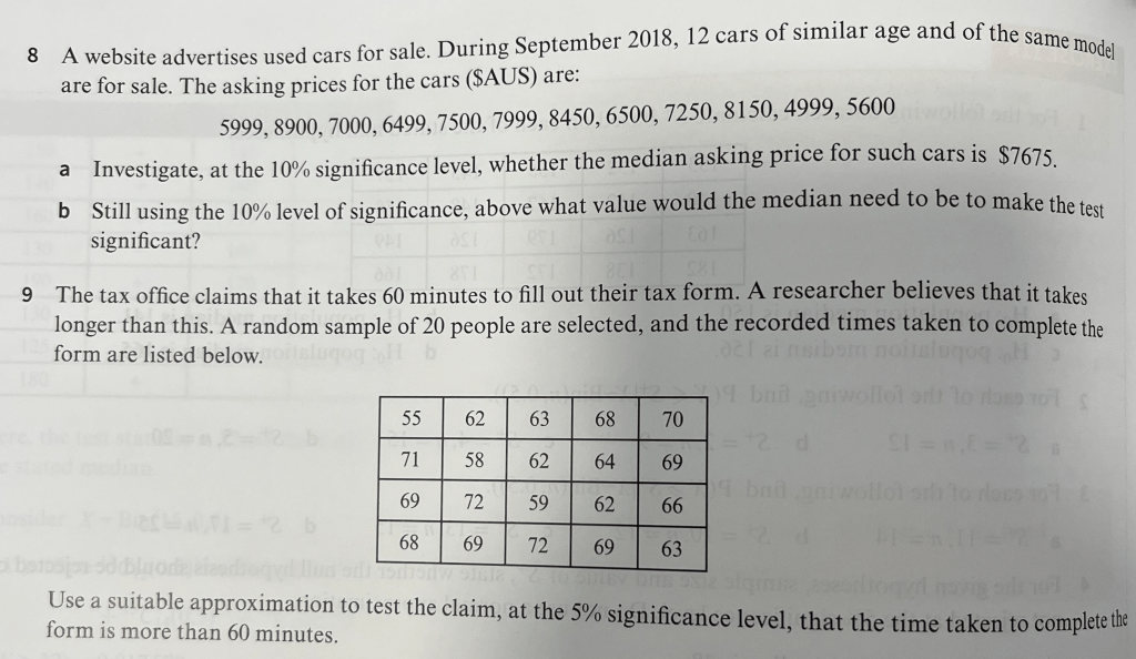
Exercise 1
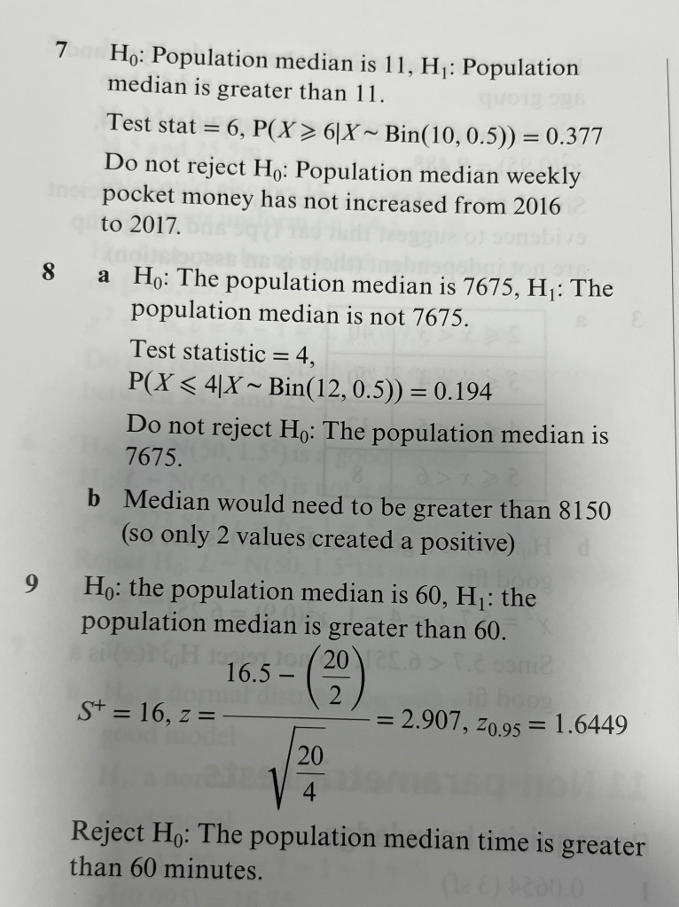
Answers to Exercise 1

Worked Solutions to Exercise 1
Single-sample Wilcoxon signed-rank Test
If the underlying data is known to be symmetric, the Wilcoxon signed-rank test is better to use as it ranks the data.
We rank each data point based on how far it is from the stated population median. The test statistic, T, is the smaller value of the sum of the negative ranks, N, and the sum of the positive ranks, P, i.e. T = min(P,N). (N.B. Two data points being an equal distance from the median (i.e. above and below) is a situation not covered in our course, but would be allocated an equal rank (e.g. if both 4th place, would both be allocated 4.5).
Although the data is continuous, the sum of ranks is discrete, and so the distribution of T is discrete. We should also note that P will be between 0 and 
Note, we have a table in MF19 that we can use to identify the critical value.
Worked Example. Single-sample Wilcoxon signed-rank Test
The kilogram weight of ten randomly selected mackerel are as follows: 1.6, 1.1, 2.1, 2.4, 2.2, 2.9, 2.6, 2.3, 2.7 and 1.9.
Test at the 5% significance level whether the median weight is greater than 1.8kg.
For large n, we can also approximate the Wilcoxon signed-rank test to a normal distribution. Given the statistic T = min (P,N), 


We use a continuity correction, as we are approximating a discrete distribution with a continuous distribution. Our z-value is:

Worked Example. Single-sample Wilcoxon signed-rank Test (Normal Approximation)
In a clinical trial, the survival time, in weeks, for 19 patients with non-Hodgkin’s lymphoma are as detailed below:
| 37 | 54 | 73 | 89 | 94 | 110 | 112 | 123 | 129 | 132 |
| 148 | 151 | 173 | 189 | 201 | 204 | 213 | 276 | 281 |
Test at the 5% significance level whether the median differs from 150.
Exercise 2
- Assuming that a Wilcoxon signed-rank test is appropriate for the data, calculate T (the test statistic) based on the null hypotheses stated:
| 67 | 71 | 72 | 75 | 77 |
| 81 | 88 | 90 | 91 | 92 |
| 94 | 97 | 102 | 104 | 105 |
(a.) H0: Population median is 85; (b.) H0: Population median is 100; (c.) H0: Population median is 70.
2. For each sample size and significance level given, state the critical value for a Wilcoxon signed-rank test.
(a.) n=8, 5% significance, one-tailed; (b.) n=15, 1% significance, one-tailed; (c.) n=18, 2% significance, two-tailed; (d.) n=9, 10% significance, two-tailed.
3. State the assumptions required for the use of the Wilcoxon signed-rank test.
4. For each of the following tests, find E(T), Var(T) and the test statistic when approximation to the normal distribution. Also state whether you would reject or not reject the null hypothesis.
a.) H0: The population median is 142.1, H1: The population median is less than 142.1, 5% significance level, T = 175, n = 30.
b.) H0: The population median is 40.6, H1: The population median is not 40.6, 10% significance level, T = 59, n = 20
c.) H0: The population median is 16.3, H1: The population median is greater than 16.3, 2.5% significance level, T = 260, n = 40.
5. A psychology student carries out a test on short-term memory. She shows 20 commonly used words to ten 18-year old males. As soon as the 20 words have been shown, the psychologist asks the participants to write down as many words as they can remember in five minutes. The sample of 18-year old males can be seen as representative of the population of 18-year old males.
The number of words correctly remembered by the participants are: 15. 7. 12. 14. 11. 10. 4. 13. 9. 2
The median number of words remembered by 65 year old males in this test is 4. Carry out a Wilcoxon signed-rank test, at the 5% level of significance, to investigate whether the median number of words remembered by the 18-year old males is greater than that for the 65-year old males.
6. Trials are carried out on a new table to ease joint pain for people with chronic arthritis. A randomly selected sample of eight patients who have been suffering from arthritis are given the new tablets. Each participant measures the time it takes for the pain to stop after taking a new tablet as soon as they wake in the morning. The times in minutes are: 34, 44, 25, 30, 8, 27, 41, 31.
The average waiting time for the old type of tablet is 43 minutes after waking.
a. Carry out a Wilcoxon signed-rank test, at the 5% significance level, to investigate whether the new tablets offer faster pain relief.
b. Give a reason why the Wilcoxon signed-rank test may be preferred to a sign test.
7. The student council of a large school believes that the average time that A-level students spend on individual study has increased because students are more aware of the need to achieve high grades. In 2018 the average time per week of the school term that students spent on individual study was 11.2 hours.
A random sample of ten students are asked to record the amount of time on individual study for three weeks during October 2016. The average times, in hours, per week are then calculated: 12, 13.2, 14.1, 10.8, 9.6, 11.3, 17.6, 14.3, 12.1, 19.2.
Test, at the 5% level of significance, whether the average amount of time spent on individual study has increased from 2015.
8. Managers at a busy international airport are studying the times taken by arriving passengers to pass immigration, collect their luggage, then pass through customs. It is known that in the past this was 50 minutes. Some changes have been made to the queuing system in the hope of reducing this time. A random sample of 45 arriving passengers is taken and the rank sums calculated as P = 55, N = 1410. Using a suitable approximation, test, with a 1% significance level, whether the median waiting time has reduced.
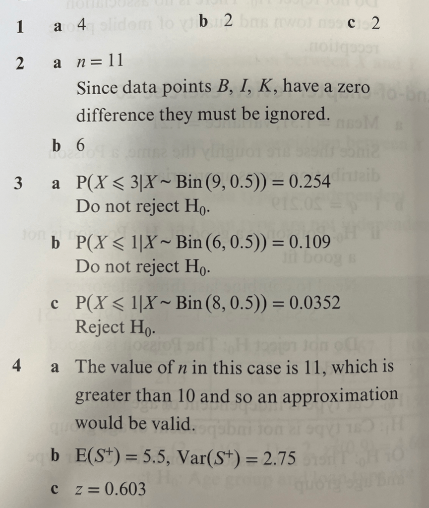
Exercise 2. Answers
- (a) P = 70, N = 50, T = 50, (b) P = 8, N = 112, T = 8, (c) P = 117, N = 3, T = 3
- (a) 5, (b) 19, (c) 32, (d) 8
- The underlying data are symmetric, the underlying data are continuous, the data are independent
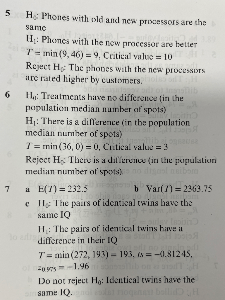
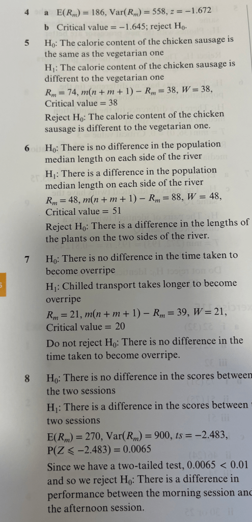
- (a) E(T) = 232.5, Var(T) = 2363.75, z = -1.172, Do not reject H0, (b) E(T) = 105, Var(T) = 717.5, z = -1.699, Reject H0, (c) E(T) = 410, Var(T) = 5535, z = -2.009, Reject H0.
- H0: The population median is 4, H1: The population median is greater than 4. T = 4, Critical value = 10. Reject H0, the population median is greater than 4.
- (a) H0: The population median is 43, H1: The population median is below 43. T = min (1,35) =1 1, Critical value = 8, Reject H0, the population median is below 43. (b) Wilcoxon signed-rank is preferred because the magnitudes of the differences are taken into account.
- H0: The population median is 11.2, H1: The population median is greater than 11.2. T = min(7,48) =7, Critical value = 10, reject H0, the population median is 11.2.
- H0: The population median is 50, H1: The population median is less than 50, T = 55, E(T) = 517.5, Var(T) = 7848.75.
, z = -5.215, z0.99 = -2.326. Reject H0, the population median is less than 50.
Two Sample Tests
The paired-sample sign test extends the idea of the sign test by looking for a positive or negative difference. In other respects it works the same as the sign test.
Worked Example – Paired-sample sign test
Data is collected on the time, in seconds, that it takes nine children to tie up their left shoelace and their right shoelace:
| Child | Left | Right |
| A | 42 | 45 |
| B | 38 | 36 |
| C | 51 | 52 |
| D | 42 | 39 |
| E | 31 | 35 |
| F | 48 | 49 |
| G | 61 | 62 |
| H | 38 | 39 |
| I | 44 | 45 |
Test at the 10% significance level whether there is a difference in the time it takes for the children to tie each shoelace.
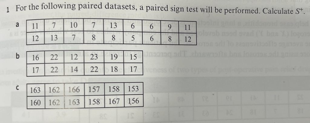
Exercise 3


Answers to Exercise 3
Worked Solutions to Exercise 3
Wilcoxon Matched-pairs signed-rank test
If we can assume that the differences in pairs of data are symmetric, then we can use the Wilcoxon matched-pairs signed-rank tests, following the same procedure as for the single sample Wilcoxon signed-rank test, testing to see whether the paired-difference median is zero.
Worked Example: Wilcoxon matched-pairs signed-rank test
An investigation is carried out into the effectiveness of two types of post-operative pain relief drug: Drug 1 and Drug 2. Seven adults agree to take Drug 1 on one day, and Drug 2 on the second. The time, in hours, of pain relief is recorded.
| Drug 1 | Drug 2 | |
| A | 4.1 | 3.9 |
| B | 3.2 | 3.3 |
| C | 5.3 | 5.0 |
| D | 5.1 | 4.6 |
| E | 4.2 | 4.6 |
| F | 3.8 | 3.2 |
| G | 3.6 | 4.3 |
Test, using the matched-pairs Wilcoxon signed-rank test, at the 5% significance level, whether drug 2 gives longer pain relief than drug 1.
Exercise 4

Answers – Exercise 4
Wilcoxon Rank-Sum test
We can only use matched-pairs testing if the data is in groups of equal size and can be paired. If we have two independent datasets of different sizes and want to test for a difference between their medians we can use the Wilcoxon rank-sum test, which has a similar design to the independent t-test.
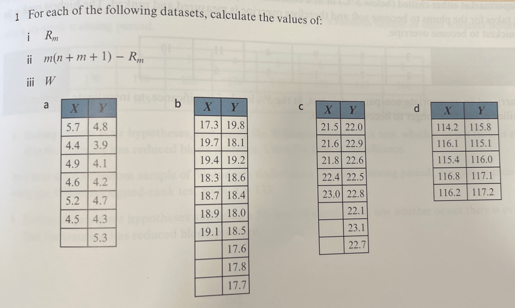
First we rank all of the data as if it were from a single population. We then take separate sums of ranks for each group. The sum of the sample with m items of data is Rm and the sum of the sample with n items of data is Rn (where m ≤ n). The test statistic that we use is W = min (Rm , m(n+m+1) – Rm) (N.B. this is in MF19).
We have separate tables in MF19 for the Wilcoxon Rank-Sum Test.
Worked Example: Wilcoxon rank-sum test
Researchers are investigating the effect of vitamin B12 on the size of the brain. A sample of males aged between 25 and 40 years is selected. Nine of them are known to have low B12 levels and seven are known to have high B12 levels. After a brain scan, the ratio of brain volume to skull capacity is recorded.
| Low B12 levels | 0.795 | 0.798 | 0.802 | 0.805 | 0.806 | 0.807 | 0.808 | 0.81 | 0.812 |
| High B12 levels | 0.786 | 0.789 | 0.792 | 0.796 | 0.799 | 0.8 | 0.803 |
Carry out a Wilcoxon rank-sum test, at the 5% significance level, to see whether the level of vitamin B12 affects the size of the brain.
Normal approximation
If m and n are large (both ≥ 10), W can be approximated as a normal distribution, with 


Worked Example: Wilcoxon rank-sum test – Normal Approximation
A company is investigating a new production technique to improve the quality of camera lenses for a phone. Samples of the lenses are given to a camera expert who is asked to rank the lenses, with rank 1 being the highest quality. The expert does not know which production technique has been used.
| Lens | A | B | C | D | E | F | G | H | I | J | K | L |
| Method | old | new | new | old | old | new | old | new | old | old | old | new |
| Rank | 12 | 1 | 2 | 9 | 10 | 5 | 21 | 6 | 20 | 22 | 23 | 17 |
| Lens | M | N | O | P | Q | R | S | T | U | V | W | X |
| Method | new | new | old | old | old | new | old | new | old | new | new | old |
| Rank | 14 | 13 | 3 | 4 | 19 | 11 | 24 | 16 | 18 | 8 | 7 | 15 |
Using a suitable approximation, test at the 5% significance level whether there is a difference in the quality of the production techniques.
Exercise 5


Answers to Exercise 5

End of “Non-Parametric Tests” Chapter Mixed Exercises

Worked Solutions to Exercise 5
Answers to End of “Non-Parametric Tests” Chapter Mixed Exercises


