9231. Statistics. Inferential Statistics

The t-distribution

In order to use a normal distribution to model data, we need to make certain assumptions.

First, we assume that either the population variance 𝞼² is known, or that the sample size is big enough that we can reasonably use the unbiased estimator of the variance s² instead.

If the sample size is small, then it isn’t appropriate to use s². In this case the t-distribution is more appropriate than the normal distribution.

The diagram below shows the t-distribution, similar to the standardised normal distribution, but with a relatively higher probability density in the tails.

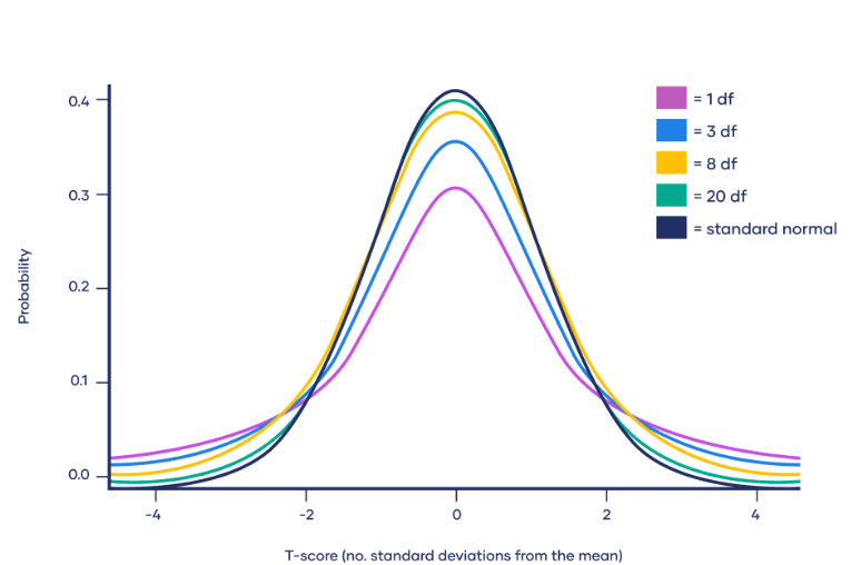
As indicated the t-distribution is actually a family of distributions with (n-1) degrees of freedom, where n is the sample size. Clearly as n increases, the t-distribution becomes more like the normal distribution.

Calculating the unbiased estimator of variance s²

Note that in some textbooks s² is called $\hat{\sigma}^2$ . Putting a hat on a parameter gives an estimator for that parameter. In this course though, s² will be used.

For a sample of size n, we calculate the unbiased estimator of the variance as

s² = $\frac{s_{xx}}{n-1}$ ,

where $s_{xx} = \Sigma (x - \bar{x})^2 = \Sigma x^2 - \frac{ (\Sigma x)^2}{n}$

Worked Example: Unbiased Estimator of Variance

The wingspans of six butterflies are measured (in cm) and recorded as: 8.8, 9.6, 9.2, 9.1, 9.9 and 8.7.

Calculate the unbiased estimate for the variance of butterfly wingspan.

Hypothesis Testing

We can use the unbiased estimator of variance to perform hypothesis tests regarding the population mean. We follow the below steps to do this

1.) We define a null hypothesis, H₀. This is the assumed value of the parameter that we are testing. So in this case we will have H₀: μ = k, where k is the assumed value of the mean we are testing.

2.) We suggest an alternative hypothesis, H₁. This may be one-tailed (e.g. larger than the assumed value) of two-tailed (i.e. different to the assumed value). So we will have either H₁: μ < k, or H₁: μ > k or H₁: μ ≠ k.

3.) We then perform a test to see whether or not we reject H₀. To perform the test, we use a t-distribution with (n-1) degrees of freedom to identify the critical value. We use the test statistic: $\frac{ \bar{x} - \mu}{\frac{s}{\sqrt{n}}}$ , with $\bar{x}$ being the sample mean and s being the unbiased estimator of standard deviation, i.e. $s = \sqrt{\frac{s_{xx}}{n-1}}$ .

To assess whether or not to reject the null hypothesis, we compare the test statistic with the critical value that we get from the t-tables in MF19. If the test statistic is “further out” than the critical value, then we can reject the null hypothesis.

For a one-tailed test at significance level 𝛼%, the critical value is t_1-𝛼,n-1. For a two-tailed test it is t_1-𝛼/2,n-1.

Worked Example – t-test

Butterflies are being bred on a farm. They should grow to have a mean wingspan of 9.4cm, however the breeders are worried that they are not growing adequately, so they take a sample of six and measure their wingspans in centimetres. The measurements are: 8.8, 9.6, 9.2, 9.1, 9.9 and 8.7. Under the assumption that the wingspans are normally distributed and using a 10% significance level, test whether the mean wingspan of the butterflies is less than 9.4cm

Worked Example – Two tailed t-test

A random sample of 12 workers from a mobile phone assembly line was selected from a large number of workers. A manager asked each of the workers to assemble a phone at their normal working speed. The times taken in minutes to assemble the phone were: 43.2, 41.6, 49.3, 48.2, 44.2, 40.6, 39.7, 43.4, 44.9, 45.1, 46.2 and 43.2.

Assuming that the sample comes from an underlying normal population, investigate the claim that the population mean is 45 minutes, using a 5% significance level.

Note, that if the sample size is large, which we take to mean 30 or more, then instead of using a t-test it is better to simply use the normal distribution directly.

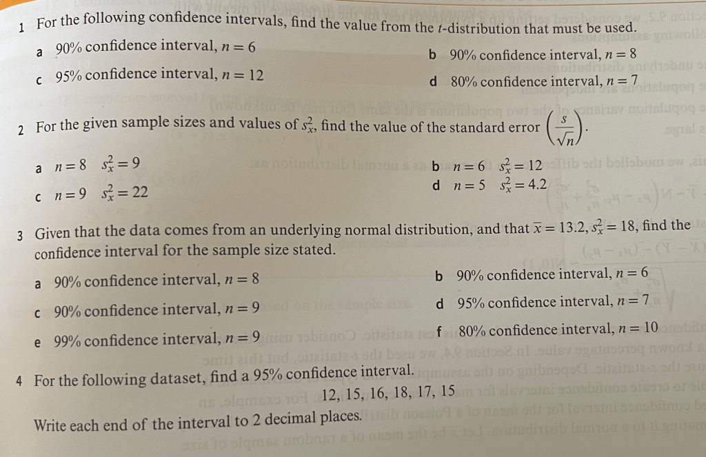
Exercise 1

1.) For the given data, find unbiased estimates for the mean and variance:

(a) 12, 16, 17, 19, 13, 14, 11, 16, 19, 21, 14, 15;

(b) 143, 154, 156, 145, 144, 132, 135, 148, 171, 124

2.) In each case, state the magnitude of the test statistic for the given value of n and stated significance level:

(a) n = 11, one-tailed 5%

(b) n = 21, one-tailed 2.5%

(d) n = 25, two-tailed 1%

(e) n = 8, one-tailed 10%

(f) n = 18, two-tailed 10%

3.) State the null and alternative hypotheses for the following tests:

(a) The population mean differs from 41;

(b) The population mean is greater than 7.3;

(d) The population mean has not changed from 6.5.

4.) For the given test statistic, sample sizes and significance levels, state whether you would reject or not reject the null hypothesis:

(a) Test statistic = 1.96, n = 10, 5% one-tailed;

(b) Test statistic = -2.764, n = 8, 1% one-tailed;

(d) Test statistic = -2.341, n = 11, 5% two-tailed;

5.) In a given week, 12 babies are born in a hospital. Assume that this sample came from an underlying normal population. The length of each baby is routinely measured and is listed below (in cm):

49, 50, 45, 51, 47, 49, 48, 54, 53, 55, 45, 50

(a) Find unbiased estimators for the mean and variance.

The average length of babies is through to be 50.5cm. There is a concern that this is an overestimate.

(b) Test this claim at the 5% significance level based on this sample.

6.) A drugs manufacturer claims that the amount of paracetamol in tablets is 60mg. A sample of ten tablets is taken and the amount of paracetamol in each is recorded:

59.1, 59.7, 61.0, 59.1, 60.6, 68.9, 60.2, 58.6, 58.6, 58.9

Assuming that this sample came from an underlying normal population, test the claim at the 5% significance level that the amount is different from 60mg.

7.) The weight, Xg, of a large bag of crisps is said to be normally distributed with a mean of 175g. A sample of eight bags is opened and the contents weighed. The results are listed below.

173.2, 171.5, 176.3, 175.1, 174.7, 174.2, 176, 174.5

A consumer group believes the bags are underfilled.

a.) Test this claim at the 5% significance level.

b.) Suggest why only a small sample of packets was tested.

8.) At a petrol station, the manager thinks that one of the pumps is not working properly and is giving out more petrol than it should. She decides to test this claim by filling up ten buckets with 5 litres, according to the pump. The results in cm³, are given below (1 litre = 1000 cm³).

It is assumed that the amounts given are from a normal distribution.

5001, 5002, 5009, 4996, 4997, 5001, 5003, 5006, 5013, 5013

Using this sample, test at the 5% significance level whether or not the petrol pump is giving out too much petrol.

Answers to Exercise 1

1.) (a) $\overline{x} = 15.583$ , s² = 9.174, (b) $\overline{x} = 145.2$ , s² = 177.96

2.) (a) t_0.95,10 = 1.812, (b) t_0.975,20 = 2.086, (c) t_0.975,14 = 2.145, (d) t_0.995,24 = 2.797, (e) t_0.9,7 = 1.415, (f) t_0.95,17 = 1.740

3.) (a) H₀: $\mu = 41$ , H₁: $\mu \neq 41$

(b) H₀: $\mu = 7.3$ , H₁: $\mu > 7.3$

(d) H₀: $\mu = 6.5$ , H₁: $\mu \neq 6.5$

4.) (a) t_0.95,9 = 1.833; reject;

(b) t_0.99,7 = 2.988; do not reject;

(d) t_0.975,10 = 2.228; reject.

5.) (a) $\overline{x} = 49.7$ , s² = 10.42

(b) H₀: $\mu = 50.5$ , H₁: \mu < 50.5 , t = -0.894, t_0.95,11 = -1.796. Do not reject H₀: The mean length is 50.5cm, based on this sample.

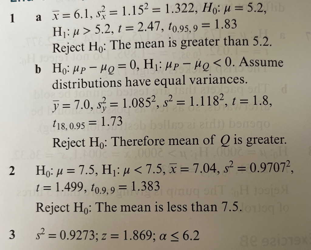
6.) Refer to worked solutions below.

7.) (a) H₀: $\mu = 175$ , H₁: $\mu < 175$ , $\overline{x} = 174$ , s² = 2.377, t = -1.032, t_0.95,7 = -1.895. Do not reject H₀: The crisp packets weight 175g.

(b) The packets that are tested cannot be sold afterwards, so as few as possible should be opened (this is called destruction testing).

(8.) H₀: $\mu = 5000$ , H₁: $\mu > 5000$ , $\overline{x} = 5004.1$ s² = 36.32, t = 2.151, t_0.95,9 = 1.83. Reject H₀: The pump is giving more that 5 litres of petrol.

Worked Solutions to Exercise 1

Hypothesis Testing: Difference between Means

We can test to see if two different populations have equal means.

To do this we must be able to assume that:
- The underlying distributions are normal;
- The populations are independent; and
- The population variance (which may be unknown) is the same in both populations.

The test statistic that we use for the difference in means is the z-value, which is distributed N(0,1) and is given by $Z = \frac{(\bar{X} - \bar{Y}) - (\mu_x - \mu_y)}{\sqrt{\frac{\sigma_x^2}{n_x} + \frac{\sigma_y^2}{n_y} }}$

Worked Example

A group of 50 children and 70 adults participate in a maths activity. The mean time taken for the children to complete the activity is 45.3 seconds, with a standard deviation of 3.2 seconds. For the adults, the mean time is 46.1 seconds with a standard deviation of 2.8 seconds. Assuming the completion times are normally distributed with equal variances, test at the 5% significance level whether or not the children are faster at completing the activity.

(N.B. In 9709:S2 we learned that a 5% significance level test on the normal curve includes 2.5% on each end of the curve, so the one-sided test actually takes the critical value for 97.5%)

Two Sample Tests

Sometimes we have two separate samples, which individually are each too small to use as estimators. We can pool them to give a pooled estimator for the variance as:

$s_p^2 = \frac{\Sigma(x - \bar{x})^2 + \Sigma(y - \bar{y})^2}{n_x + n_y -2} =\frac{(n_x - 1)s_x^2+(n_y - 1)s_y^2}{n_x +n_y -2}$ , where $s_x^2 = \frac{\Sigma(x-\bar{x})^2}{n_x-1}$ and $s_y^2 = \frac{\Sigma(y-\bar{y})^2}{n_y-1}$

N.B. As previously, $\Sigma (x - \bar{x})^2 = \Sigma x^2 - \frac{ (\Sigma x)^2}{n_x}$ and $\Sigma (y - \bar{y})^2 = \Sigma y^2 - \frac{ (\Sigma y)^2}{n_y}$

In this case, as we assume that the variances are equal and also equal to the pooled estimator, the test statistic $Z = \frac{(\bar{X} - \bar{Y}) - (\mu_x - \mu_y)}{\sqrt{\frac{\sigma_x^2}{n_x} + \frac{\sigma_y^2}{n_y} }}$ becomes $T = \frac{(\bar{X} - \bar{Y}) - (\mu_x - \mu_y)}{\sqrt {s_p^2(\frac{1}{n_x} + \frac{1}{n_y} )}}$ , with critical value $t_{1 - \alpha , n_x + n_y - 2}$ or $t_{1 - \alpha /2 , n_x + n_y - 2}$

N.B. When pooling data we typically consider sample size to be small if n<15 (an indicator that the CV should come from the t-distribution).

Worked Example: Pooled data

A shopkeeper believes that playing music in the shop encourages customers to spend more money. To test his belief, he records how much money is collected during a ten-day period when music is playing and then during an eight-day period when music is not playing. His sales, in thousands of dollars, are detailed below:

With music	Σx = 960.1	Σx² = 92,274.44
Without music	Σy = 748.2	Σy² = 70,041.16

If we assume that the data are randomly sampled from normal distributions with the same variance, test the shopkeepers claim, using a 5% significance level.

Exercise 2

1.) Given the sample variance and sample size of each set of data, find the pooled estimate of variance.

(a) s_x² = 13.2, n_x = 15, s_y² = 11.9, n_y = 13;

(b) s_x² = 161.2, n_x = 21, s_y² = 158.7, n_y = 24;

(b) s_x² = 32.1, n_x = 60, s_y² = 48.6, n_y = 40;

2.) For the following pairs of data sets, find an estimate for the pooled variance:

(a) X:

27	19	15	19	21
18	17	16	20	28

32	31	27	26
29	30	28	14

(b)

23	25	26	19	22	21
28	25	26	19	23

14	19	21	20	17
16	18	15	21

3. For each question, state the magnitude of the test statistic for the given values of n_x and n_y and state the significance level.

(a) n_x=8, n_y=6, one-tailed 5%;

(b) n_x=14, n_y=10, one-tailed 2.5%;

(d) n_x=20, n_y=12, two-tailed 1%;

(e) n_x=11, n_y=14, one-tailed 10%;

(f) n_x=17, n_y=12, two-tailed 10%.

4.) For each of the following, state the null and alternate hypotheses.

(a) The difference in population means is not 0;

(b) The population mean for X is greater than the population mean for Y;

(d) The difference in the population means is not six units.

5.) Two examiners are marking an examination paper, and it is believed that examiner A is more strict than examiner B. The results from several papers are added together for each examiner, and presented in the following table:

	Sample Size	Sum of Marks
Examiner A	16	689
Examiner B	12	636

Test the claim at the 5% significance level, assuming that the marks are normally distributed with a standard deviation of 15.

6.) Takahe birds are native to New Zealand and are very rare. The male birds and female birds look very similar. The only way of differentiating males from females is to measure their weights. It is known that the female bird is slightly smaller than the male, and so weighing them could be a way of identifying the gender of an adult Takahe bird.

The weights of ten male and eight female Takahe birds are measured, and the summative statistics are presented in the following table:

	Sample Size	Sum	Sum of squares
Male	10	28.1	79.4
Female	8	21.5	58.3

(a) Find s_p², the pooled estimator of the population variance.

(b) Test, at the 5% significance level, whether male Takahe birds are heavier than female Takahe birds assuming the weights are normally distributed.

7.) A company that makes computers must transport them from its warehouse to the delivery centre, with one lorry delivery per day. In three weeks’ time, the usual rout will have roadworks stopping the traffic for six weeks. The local council says that the alternative route will add not more than ten minutes to the route. The manager of the company does not think that this is true and so, for the next 14 days, he asks eight of the company’s lorry drivers to travel the new route, and six to travel the old route.

Old	34	45	36	47	42	43
New	47	51	47	50	53	51	50	45

8.) Samples are taken from two different types of honey and the viscosity (i.e. how “runny” the honey is) is measured.

Honey	Mean	Standard deviation	Sample size
A	114.44	0.62	4
B	114.93	0.94	6

Assuming normal distributions, test at the 5% significance level whether there is a difference in viscosity between the two types of honey.

Exercise 2: Answers

1.) (a) s_p² = 12.6, (b) s_p² = 159.86, (c) s_p² = 38.67

2.) (a) s_p² = 24.68, (b) s_p² = 7.746

3.) (a) t_0.95,12 = 1.782, (b) t_0.975,22 = 2.074, (c) t_0.975,13 = 2.160, (d) t_0.995,30 = 2.750, (e) t_0.9,23 = 1.319, (f) t_0.95,27 = 1.703

4.) (a) H₀: $\mu_x - \mu_y = 0$ H₁: $\mu_x - \mu_y \neq 0$ , (b) H₀: $\mu_x - \mu_y = 0$ , H₁: $\mu_x - \mu_y > 0$ , (c) H₀: $\mu_x - \mu_y = 5$ , H₁: $\mu_x - \mu_y > 5$ , (d) H₀: $\mu_x - \mu_y = 6$ , H₁: $\mu_x - \mu_y \neq 6$

5.) NB: we are give $\sigma = 15$ , H₀: $\mu_A - \mu_B = 0$ , H₁: $\mu_A - \mu_B < 0$ . (If more severe, A should be giving fewer marks on average). Test statistic = -1.7348, z = -1.96. Do not reject H₀: Examiner A is not more severe than examiner B.

6.) (a) s_p² = 0.0599 (4 decimal places)

6.) (b) H₀: $\mu_M - \mu_F = 0$ , H₁: $\mu_M - \mu_F > 0$ , t = 1.056, t_0.95,16 = 1.746. Do not reject H₀: Male Takahe birds are not significantly heavier than female Takahe birds.

7.) (a) s_p² = 15.03

7.) (b) H₀: $\mu_N - \mu_O = 10$ , H₁: $\mu_N - \mu_O > 10$ , t = -0.915, t_12,0.95 = -1.782. Do not reject H₀: The council is correct in stating that the new route will not add more than ten minutes to the journey.

8.) H₀: $\mu_B - \mu_A = 0$ , H₁: $\mu_B - \mu_A \neq 0$ , t = 0.91, t_0975,8 = 2.306. Do not reject H₀: There is no difference in the viscosities of the two types of honey.

Exercise 2: Worked Solutions

Paired t-tests

So far we have compared the means in two different samples. This is sometimes called an unpaired test as there is no natural “pairing” between the samples.

In situations such as “before and after” there is a natural pairing between the two datasets. In this case it is more appropriate to use a paired t-test. In this case, instead of measuring the difference in the means, we measure the mean of the differences.

The test statistic for a paired t-test with sample size n and null hypothesis μ_d = k (often with k = 0) is $\frac{ \bar{d} - k}{ \frac{s_d}{\sqrt{n}}}$ , where d_i=x_i-y_i and $\bar{d}$ and s_d are the sample mean and standard deviation of $D \sim N(\mu_d , \frac{s_d^2}{n} )$ . We test using a t-distribution with n-1 degrees of freedom.

Worked Example: Paired t-test for “before and after” data

A diagnostic test is taken by ten students before a revision session and then again after completing the revision session. Their scores are presented in the following table:

Student	A	B	C	D	E	F	G	H	I	J
Before	45	54	49	51	53	64	71	55	78	43
After	49	56	56	54	61	70	72	60	82	51

Using a paired t-test, and assuming the differences in scores are normally distributed, test at the 5% significance level whether the revision was effective.

Worked Example: Paired t-test for “before and after” data – testing for difference from mean

Using the same scenario and data as in the previous example, use a paired t-test, assuming that the differences in scores are normally distributed, to test at the 5% significance level whether students have increased their scores by four marks or more.

Exercise 3

1.) For each of the following pairs of data, find the sample mean of the difference, $\overline{d}$ , and the unbiased estimator of the variance of the distance, s_d².

(a)

X	124	139	128	119	119	112	113	128	113
Y	127	117	121	126	119	125	118	118	127

(b)

X	34.3	30.8	32.8	27.5	26.3	27.8	35.1	31.1	28.5	31.5	30.7	29.5
Y	27.3	28.5	30.5	29	28	33	31.6	28	32.8	28.1	30.9	30

(c)

X	75	84	80	66	78	97	68	86	86	73	97	70	72
Y	81	81	86	90	87	76	88	89	84	92	85	90	91

2.) For the given null hypotheses, find the test statistic of the following summative data.

(a) $H_0: \mu_d = 0$

$\mu_d = 0.344$ , s_d² = 121, n = 11.

(b) $H_0: \mu_d = 0$

$\mu_d = -0.688$ , s_d² = 11.62, n = 10.

$\mu_d = -5.82$ , s_d² = 182.3, n = 12.

3.) For the data in questions 2a-c, state the magnitude of critical value, given the following alternate hypothesis and significance level.

a.) H1: $\mu_d \neq 0$ , significance level 5%

b.) H1: $\mu_d > 0$ , significance level 5%

c.) H1: $\mu_d < -5$ , significance level 2.5%

4.) A biologist investigates the effect of a new food on Takahe male birds. Eight birds are weighed (in kg). They are then fed the new food for 14 days and weighed again.

Let us assume that the weight gains are normally distributed.

Initial weight (kg)	2.67	2.93	3.12	3.21	2.64	2.73	2.86	2.91
Weight after 14 days (kg)	2.71	3.01	3.19	3.24	2.6	2.78	2.84	2.97

Test, at the 2.5% significance level, to investigate whether there has been a significant increase in the weight of the Takahe male birds.

5.) A diet programme aims at trying to help people lose at least 2kg in weight within five weeks of starting the programme. A sample of eight participants are asked to volunteer to take part in the experiment and their weight at the beginning of the programme and after five weeks is measured and recorded. The following estimators were calculated: $\overline{d} = 2.225$ ; s_d² = 0.931589. Test, at the 5% significance level, the claim that participants will lose at least 2kg of weight within the first five weeks of the programme, assuming the weight losses are normally distributed.

6.) Police trainees are given a test to assess how good their memory is. After seeing ten car plates for 15 seconds each, they must write down as many as they can remember. The trainees then attend a memory improvement course. After this week-long course, they are retested. The results of the tests for eight police trainees are presented in the following table:

Number correct before course	6	5	6	5	7	5	4	6
Number correct after course	6	8	6	7	9	8	9	6

Test, at the 5% significance level, whether the course has made a difference to the trainees’ scores, assuming the differences in scores are normally distributed.

7.) A company sends its employees to a psychologist to try to improve their sales productivity. The following table shows the sales figures, in thousands of dollars, of six employees before and after seeing the psychologist.

	A	B	C	D	E	F
Before	10	8	15	38	60	90
After	14	9	16	42	80	83

Test, at the 5% significance level, whether the visits to the psychologist have improved sales productivity, assuming the increases in sales are normally distributed.

Answers to Exercise 3

Worked Solutions to Exercise 3

Confidence Intervals: Mean of a small sample

We often use confidence intervals to help with statistical inference. With confidence intervals, instead of finding a critical region we find an acceptance region.

The confidence interval is found from the sample taken. A 100(𝛼-1)% confidence interval for μ is $\bar{x} \pm ( t_{\frac{\alpha}{2},n-1} ) \frac{s}{\sqrt{n}}$

Worked Example

A random sample of people queueing for a train ticket are asked how long they have been waiting in the queue before buying their ticket. Their replies, in minutes, are 12, 17, 21, 9, 14, 19.

(a.) Assuming a normal distribution, calculate a 90% confidence interval for the mean stated waiting time.

(b.) Comment on the train company’s claim that the mean waiting time is ten minutes.

Exercise 4

Answers: Exercise 4

Worked Solutions: Exercise 4

Confidence Intervals: Difference in Means

When we looked at a hypothesis test for the difference in means, we used the following z-value as a test statistic: $z = \frac{(\bar{X} - \bar{Y})-(\mu_x - \mu_y)}{\sqrt{\frac{\sigma_x^2}{n_x} + \frac{\sigma_y^2}{n_y}}}$ , which was distributed N(0,1).

If X and Y are independent populations, both with the same (although unknown) variance, and n is large, then we can calculate a 100(𝛼-1)% confidence interval for the difference in means using $\bar{x} - \bar{y} \pm z_{\frac{\alpha}{2}} \sqrt{\frac{s_x^2}{n_x} + \frac{s_y^2}{n_y}}$

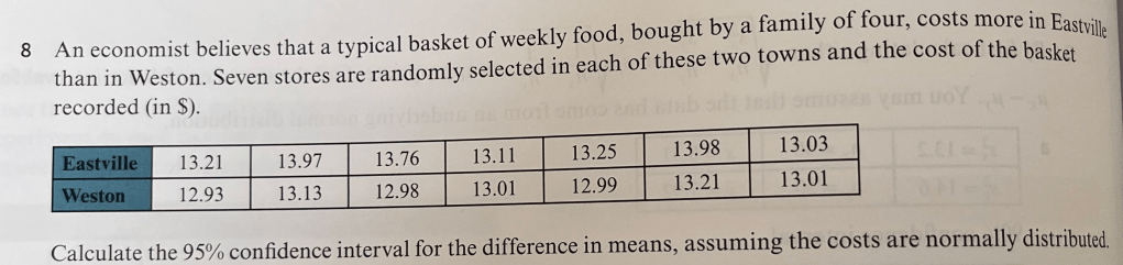
If the sample is small, i.e. n<30, then we pool the variances to get the best estimate and model the difference as a t-distribution.

Pooling the variances and letting s_p² be the pooled estimate of the population variance gives the test statistic $t_{\frac{\alpha}{2},n_x+n_y-2} = \frac{(\bar{X} - \bar{Y}) - (\mu_x - \mu_y)}{ \sqrt{s_p^2(\frac{1}{n_x} + \frac{1}{n_y})} }$

A 100(𝛼-1)% confidence interval for the difference in means for small samples is $(\bar{x} - \bar{y}) \pm t_{\frac{\alpha}{2},n_x+n_y-2} \times s_p \sqrt{\frac{1}{n_x} + \frac{1}{n_y}}$ , where $s_p^2 = \frac{\Sigma(x - \bar{x})^2 + \Sigma(y - \bar{y})^2}{n_x + n_y - 2}$ .

If we know the unbiased estimators s_x² and s_y², we can calculate s_p² using $\frac{(n_x - 1)s_x^2 + (n_y - 1)s_y^2}{n_x + n_y - 2}$

A 100(𝛼-1)% confidence interval for the difference in means for matched pairs is $\overline{d} \pm t_{ \frac{ \alpha }{2} , n-1 } \times \frac{ s_d }{ \sqrt{n}}$

Worked Example: Confidence interval for difference of means

A group of 60 men and 70 women participate in a maths activity. The mean time taken for the men to complete the activity is 45.3 seconds, with a standard deviation of 3.2 seconds. For the women, the mean time is 46.1 seconds with a standard deviation of 2.8 seconds. Assuming the completion times are normally distributed with equal variances, find a 90% confidence interval for the difference in means.

Worked Example: Changing confidence interval for difference of means

Given that a 90% confidence interval is (-0.0745, 1.6745), calculate a 99% confidence interval.

Worked Example: Confidence interval for difference of means using pooled estimate of population variance

A shopkeeper believes that playing music in his shop encourages customers to spend more money. To test this he records how much money was collected for a ten-day period whilst music was playing and then an eight-day period when it wasn’t. The sales, in thousands of dollars, are summarised below:

With music	Σx = 960.1	Σx² = 92,274.44
Without music	Σy = 748.2	Σy² = 70,041.16

Assuming that the data are randomly sampled from normal distributions with the same variance, find the 90% confidence interval for the difference in means.

Worked Example: Confidence Interval (Paired data)

A chemist has developed a fuel additive and claims that it reduces the fuel consumption of cars. Eight randomly selected cars were each filled with 20 litres of fuel and driven around a race circuit. Each car was tested twice, once with the additive and once without it. The distances in miles that each car travelled before running out of fuel are given in the table below:

Car	1	2	3	4	5	6	7	8
Distance without additive	163	172	195	170	183	185	161	176
Distance with additive	168	185	187	172	180	189	172	175

Assuming a normal distribution, find a 90% confidence interval for the difference in the distances travelled.

Exercise 5

Answers to exercise 5

Worked Solutions to Exercise 5

End of Chapter “Inferential Statistics” Exercise

Answers to End of Chapter “Inferential Statistics” Exercise

9231. Statistics. Inferential Statistics

Share this: