A random variable can be the set of possible values from a random experiment. A continuous random variable is a random variable that can take all values within an interval, e.g. time or length. An example of a continuous random variable is the time that a sample of people have to wait before their bus arrives at a certain bus stop on a certain day.
Probability Density Function
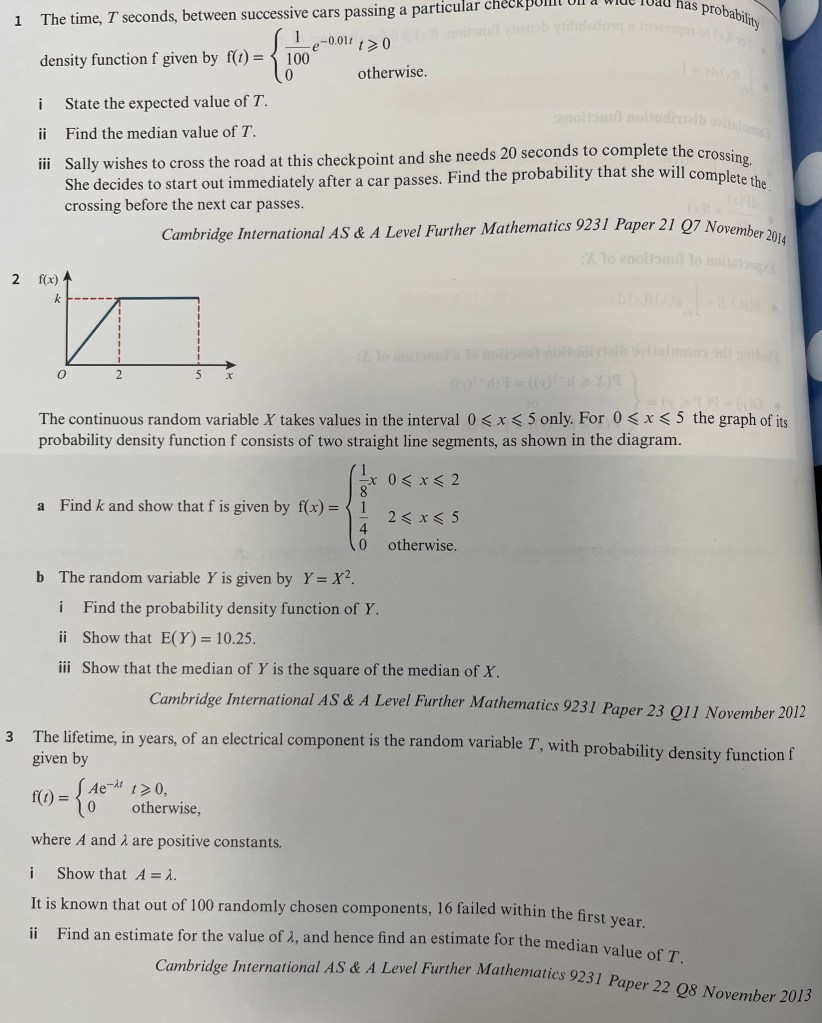
A probability density function (PDF) describes the probability of a continuous random variable (cRV) in the same way that a probability distribution table describes the probability of a discrete random variable.
The probability that a cRV takes any specific value is always equal to zero, which is why we can’t use a table, but use a function instead. Probability cannon be negative, so a PDF can never be negative (i.e. f(x)≥0 for all values of x).
As we are dealing with a function, instead of adding values to evaluate probability over an interval, we integrate the PDF between the limits being considered. The total area between the function and the x-axis over the values for which it is defined must equal 1, which is the total probability of the PDF.
Worked Example – PDF
Find the value of k for which f(x) = kx2 could represent a probability density function over the interval 1 ≤ x ≤ 3.
A PDF may be represented by a combination of different functions at different intervals, in which case we call it a piecewise function
Worked Example – Piecewise function
Consider the continuous random variable X, which has probability density function:
- f(x) =
- k(x+1) for 1 ≤ x < 4;
- k for 4 ≤ x ≤ 8;
- 0 otherwise.
(a) Find the value of k;
(b) Calculate P(2≤X<6)
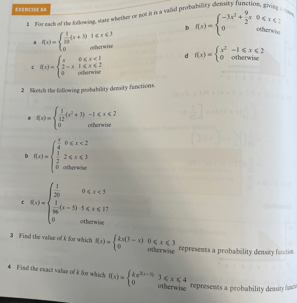
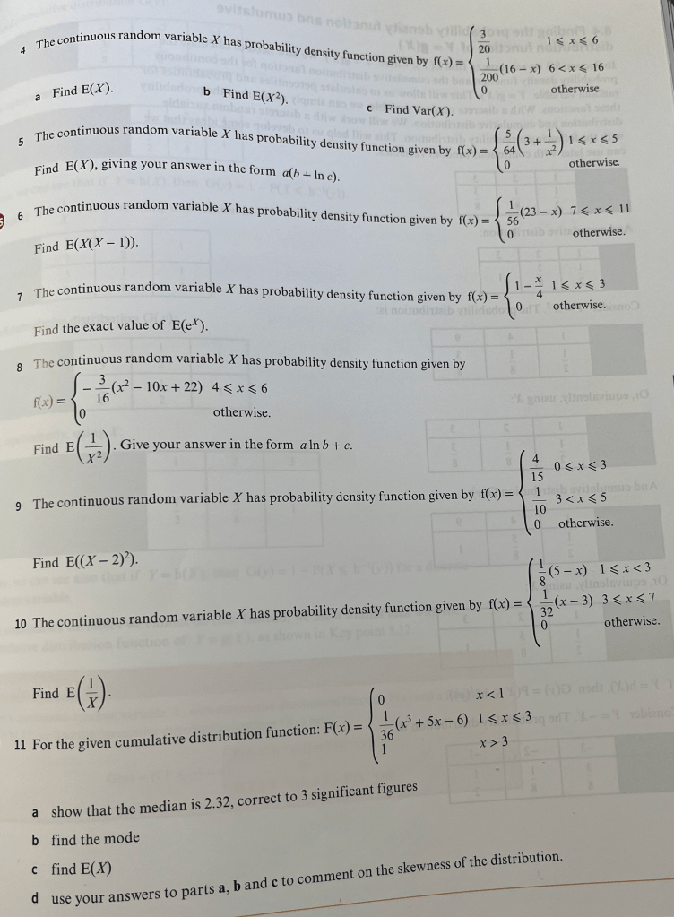
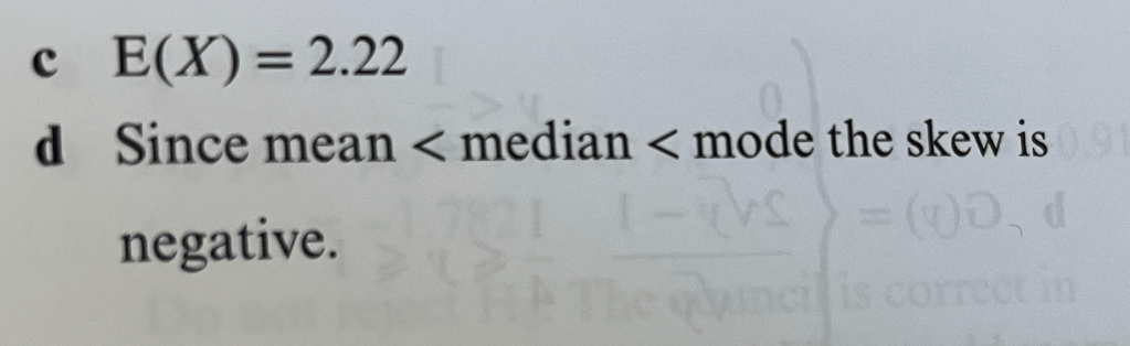
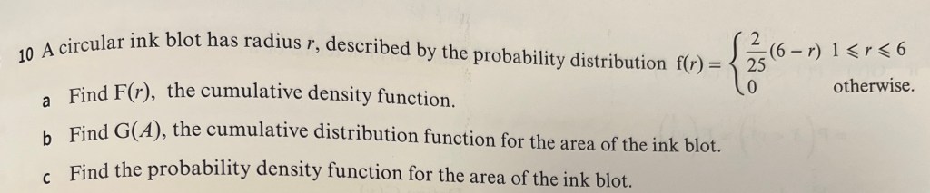
Exercise 1

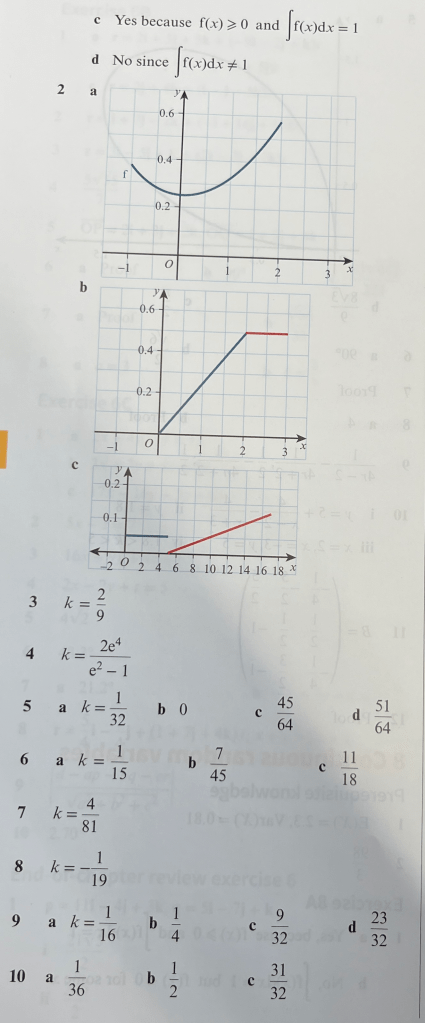
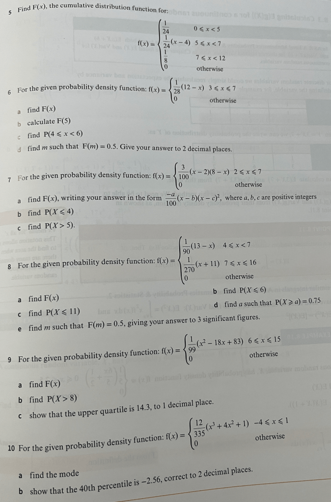
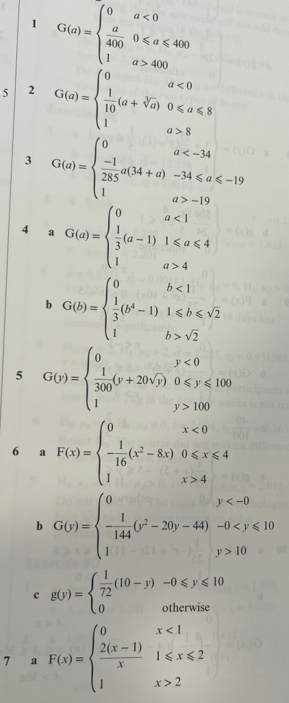
Exercise 1 Answers

Cumulative Distribution Function
Because we are often integrating the PDF (f(x)) between two limits to find the area under the curve, which is the probability, it is easier to first calculate the Cumulative Distribution Function (CDF), (F(x)) by integrating the PDF to find its primitive, which we can then substitute the limits into and take their difference.
If f(x) is a PDF, then the cumulative distribution function is defined as F(x) = P(X≤x) =

Worked Example. Cumulative Distribution Function
The continuous random variable X has probability density function 
If the PDF is piecewise defined, we need to calculated the CDF for each piece of the function and then add the probabilities. The PDF may not be continuous, but the CDF must be continous. For later “pieces” we add the cumulative probability from earlier pieces to the result of the integration.
Worked Example. Cumulative Distribution Function from Piecewise Probability Density Function
The continuous random variable X has the following probability density function:


f(x) = 0 otherwise.
(a) Find the cumulative distribution function.
(b) Find P(2 < X < 5)
(c) Find the value of a for which P(X>a) = 0.1
Percentiles
The n’th percentile, 𝝰, of a continuous random variable X, is defined as P(X≤𝝰) = n/100 (e.g. so the 95th percentile of a continuous RV is 𝝰 such that P(X≤𝝰) = 95/100.
So, if we know the CDF, the nth percentile 𝝰 is such that F(𝝰) = n/100.
The median, lower quartile and upper quartile can be thought of as important percentiles, such that F(q1) = 0.25, F(m) = 0.5 and F(q3) = 0.75.
Worked Example. Percentiles
Let X be a random variable with the following cumulative distribution function:
F(x) = 0 for x < 0

F(x) = 1 for x > 3
(a) Calculate the median
(b) Calculate the lower and upper quartiles
(c) Calculate the 40th percentile
If we are given the PDF (f(x) instead of the CDF (F(x)), we simply need to integrate it to get the CDF.
Worked Example. Percentiles from PDF
Let X be a continuous random variable with probability density function 
Show that the median is 1.52 correct to 3 significant figures.
Sometimes we need to go the other way and find the PDF from the CDF by differentiating. If the function is piecewise defined, each piece must be differentiated and applies to the same interval. We need the PDF if we want to calculate the mean or the variance, as we cannot calculate these directly from the CDF.
Worked Example. PDF from CDF
A continuous random variable, X, has the following cumulative distribution function:
F(x) = 0 for x < 0

F(x) = 1 otherwise.
Find the probability density function.
Mode
We can use the PDF to calculate the mode of a function, as this will be the highest point on the PDF (We can differentiate the PDF to help us, but take care, because the stationary point is not always the maximum point of the curve – always check the boundaries too).
Worked Example – Mode 1
For each of the following probability density functions, find the mode:
(a) 
(b) 
(c) 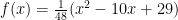
Sometimes functions can be more complicated and so it is not algebraically immediately clear where the maximum, and therefore the mode, is. In such cases it is best to draw a graph.
Worked Example – Mode 2
Given that:

f(x) = 
and f(x) = 0 otherwise, find the mode.
Exercise 2

In question 5 below, we can’t use boundary conditions for the middle piece, but we can use the fact that as the cdf must be continuous, so f(5) must give the same value in each of the first two pieces.
Answers to Exercise 2

Expectation of g(X) for a continuous random variable
If we have discrete random variables, we can calculate the expectation and variance of a function of the RV simply by redefining the variable. So if we have the following distribution for RV X:
| x | 1 | 2 | 3 |
| P(X=x) | 1/3 | 1/6 | 1/2 |
then for the RV Y = 3X+7, we can write the probability distribution as:
| y | 10 | 13 | 16 |
| P(Y=y) | 1/3 | 1/6 | 1/2 |
and use this table for Y to calculate E(3X+7) and Var(3X+7).
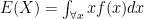
This method won’t work for continuous RVs. We must calculate E(g(X)) and Var(g(X)) from the probability density function, using:

Remember that Var(X) = E(X2) – [E(X)]2, which in this case would be

Worked Example: Expectation of Function of Continuous RV 1
A continuous RV, X, has PDF, 
(a) Find E(X)
(b) Find E(X(X+1))
Worked Example: Expectation of Function of Continuous RV 2
A continuous RV, X, has the following PDF:


Find

Exercise 3

Answers: Exercise 3

Finding the PDF and CDF of a function of a continuous RV
To understand how to deal with continuous RVs we will first look closely at the process with a discrete random variable.
We consider the following probability distribution of X:
| x | 1 | 2 | 3 |
| P(X = x) | 1/2 | 1/8 | 3/8 |
We can write the cumulative distribution for X as:
| x | 1 | 2 | 3 |
| F(x) | 1/2 | 5/8 | 1 |
We now consider Y = X2. This has the following probability distribution:
| y | 1 | 4 | 9 |
| P(Y = y) | 1/2 | 1/8 | 3/8 |
Or, we can write this using X as:
| x | 1 | 2 | 3 |
| P(X = √y) | 1/2 | 1/8 | 3/8 |
The cumulative distribution, G(y), for Y will be:
| y | 1 | 4 | 9 |
| G(y) = P(Y≤y) | 1/2 | 5/8 | 1 |
Or, again writing it using X:
| x | 1 | 2 | 3 |
| F(√y) = P(X ≤ √y) | 1/2 | 5/8 | 1 |
If Y = h(X), then G(y) = P(X ≤ h-1(y))
Y = -X has the following probability distribution:
| y | -3 | -2 | -1 |
| P(Y = y) | 3/8 | 1/8 | 1/2 |
and the following cumulative distribution:
| y | -3 | -2 | -1 |
| G(y) = P(Y ≤ y) | 3/8 | 1/2 | 1 |
Or, using X:
| x | 1 | 2 | 3 |
| F(-y) = P(X ≥ y) = 1 – P(X ≤ -y) | 1/2 | 5/8 | 1 |
We notice that if Y = h(x) then G(Y) = 1 – P(X ≤ h-1(y)).
Consider Y = 1/X. This has the following probability distribution:
| y | 1/3 | 1/2 | 1 |
| P(Y=y) | 3/8 | 1/8 | 1/2 |
and the following cumulative distribution, G(y)
| y | 1/3 | 1/2 | 1 |
| G(y) = P(Y ≤ y) | 3/8 | 1/2 | 1 |
Or, using X:
| x | 1 | 2 | 3 |
| F(1/y) = P(X ≥ 1/y) = 1 – P(X ≤ 1/y) | 1/2 | 5/8 | 1 |
We again notice for a discrete RV that if Y = h(x) then G(Y) = 1 – P(X ≤ h-1(y)).
A similar idea applies with continuous RVs:
For continuous RV X with CDF F(X) and for a function Y = h(X), we can find the CDF G(y) as follows:
G(y) = P(Y ≤ y) = P(X ≤ h-1(y)) = F(h-1(y)) or P(X ≥ h-1(y)) = 1 – F(h-1(y))
Worked Example: CDF of Function of X
Consider the continuous RV X with the following CDF:
F(x) = 0 for x < 0

F(x) = 1 for x > 4.
Find the cumulative distribution function of Y = X2.
Above we found the CDF of a function of X from the CDF of X. If we start with the PDF of X and need to find the PDF of Y=g(x), we must use the following steps:
PDF of x (f(x))
change to
CDF of X (F(x))
change to
CDF of Y (G(y))
change to
PDF of Y (g(y)).
Worked Example: PDF of function of X
A continuous random variable X has PDF 

Worked Example: PDF of 1/X
Let the continuous RV X have PDF 
Find the PDF of Y = 1/X (Hint: Taking the reciprocal changes the direction of the inequality, so F(x) becomes (1 – G(y).
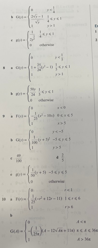
Exercise 4


Answers to Exercise 4
Worked solutions to Exercise 4
End of Chapter ‘Continuous Random Variables’ Exercise
End of Chapter ‘Continuous Random Variables’ Exercise Answers

