9231. Statistics. Chi-Squared Tests

Now we will look at tests to consider whether data fits a specific distribution. Sometimes the parameters will be known, sometimes they will be unknown. We will also look at whether two sets of data (e.g. hair colour and eye colour) are associated.

Consider rolling a dice and testing whether the values indicate that the dice is unbiased. In this case we would be considering if the data fit a discrete uniform distribution, uniform because each outcome has the same probability.

To do a hypothesis test, we would first set our null hypothesis as H₀: There is no difference between the observed data and the expected values and our alternative hypothesis as H₁: There is a difference between the observed data and the expected values.

To be more specific we can use the following null and alternative hypotheses:

H₀: A discrete uniform distribution is a good-fit model

H₁: A discrete uniform distribution is not a good-fit model

Suppose that we rolled a dice 180 times and collected the following data:

Number, n	1	2	3	4	5	6
Observed frequency	29	31	34	39	23	24

A discrete uniform distribution would have P(X=x)=1/6 ∀ x = 1,2,3,4,5,6. So the expected frequencies from this distribution can be calculated by multiplying the total frequency by the probabilities of each outcome, to give:

Number, n	1	2	3	4	5	6
Observed frequency	30	30	30	30	30	30

Note the subtle point that because we know the total frequency, and we know the expected frequencies of values 1 through 5, the expected frequency of 6 (i.e. 30) is therefore a balancing figure, meaning we don’t have to calculate it directly, but can deduce it from the others. We can say that this is not a free variable. This may not seem relevant, but we will see later that this has an impact when we calculate the test statistic. We call this situation a constraint that reduces the free variables (or degrees of freedom) in the system by one.

In general, for a goodness of fit test, we calculate the degrees of freedom, using 𝞶 = number of expected values – 1 – number of parameters estimated.

Continuing with our dice example, we now understand why the degrees of freedom, 𝞶 = 5, and we currently have the following data:

Number, n	1	2	3	4	5	6
Observed frequency (O_i)	29	31	34	39	23	24
Expected frequency (E_i)	30	30	30	30	30	30

As a test statistic we use $\chi^2(\nu) = \Sigma (\frac{(O_i - E_i)^2}{E_i})$ . Clearly this will be zero if there is no difference between the distributions.

In order to use a chi-sqared (𝟀²) test with 𝞶 degrees of freedom, we need the following conditions to be met:

Each O_i represents a frequency;
All E_i are greater than 5;
The classes all form a sample space (i.e. each observation matches only one category).

Worked Example – Chi Squared Test

An experiment is carried out to test whether or not a dice is biased. The dice is rolled 180 times, with the following results. Test at the 5% significance level whether the dice is biased:

Number, n	1	2	3	4	5	6
Observed frequency	29	31	34	39	23	24

Exercise 1

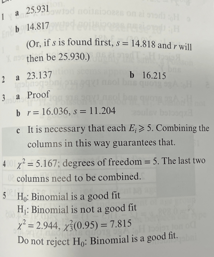
Answers to Exercise 1

Worked Solutions to Exercise 1

Goodness of Fit for Discrete Distributions (Binomial and Poisson)

We can try to see if a dataset fits well with a binomial distribution B(n,p). The probability of success may or may not be stated. If it is not stated, we use the estimator $\hat{p} = \frac{\bar{x}}{n}$ , and using the estimator reduces our degrees of freedom by 1. (N.B. We calculate the mean from the observed dataset as $\bar{x} = \frac{\Sigma r_i \times O_i}{N}$ ).

Worked Example. Goodness of Fit of Binomial Distribution

The data in the following table are thought to be binomially distributed.

x	0	1	2	3	4	5	6	7
Frequency	10	34	63	48	29	10	4	2

Test at the 5% significance level the claim that the data are binomially distributed.

Similarly with the Poisson distribution (a distribution introduced in S2 which is the probability of a given number of events occurring in a fixed interval of time or space if these events occur with a known constant mean rate) we can try to find whether a dataset fits the Poisson distribution with or without the given rate. The parameter here is 𝞴 which can be estimated with $\hat{ \lambda} = \frac{\Sigma r_i \times O_i}{N}$

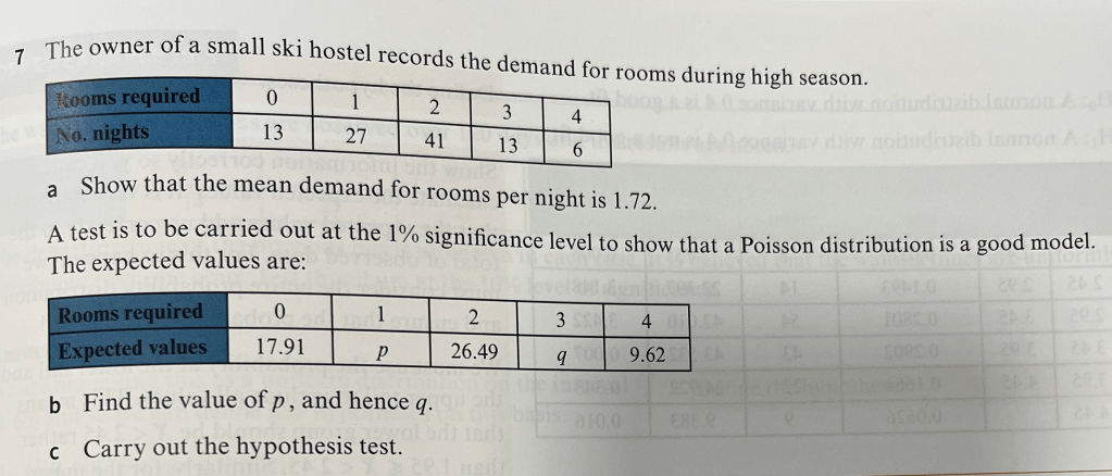
Worked Example. Goodness of Fit of Poisson Distribution

The data in the table below are thought to be modelled as a Poisson distribution with a mean of 2.5.

Number, n	0	1	2	3	4	5	6	7-
Frequency	8	34	42	28	26	5	5	2

Test the claim at the 5% level of significance that the data can be modelled as a Poisson distribution with mean 2.5.

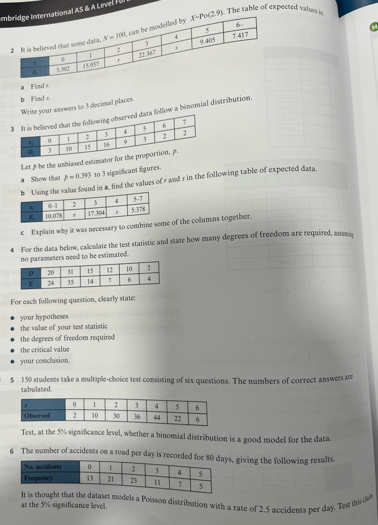
Exercise 2

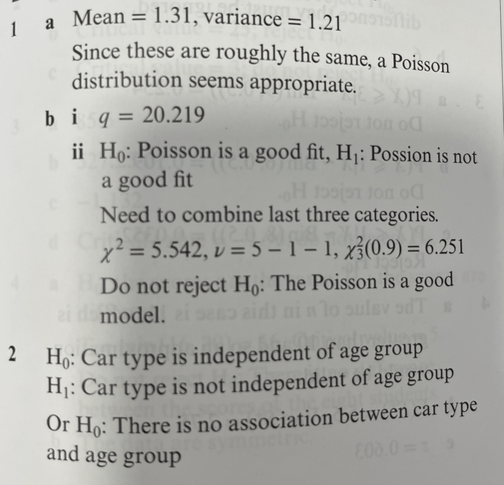
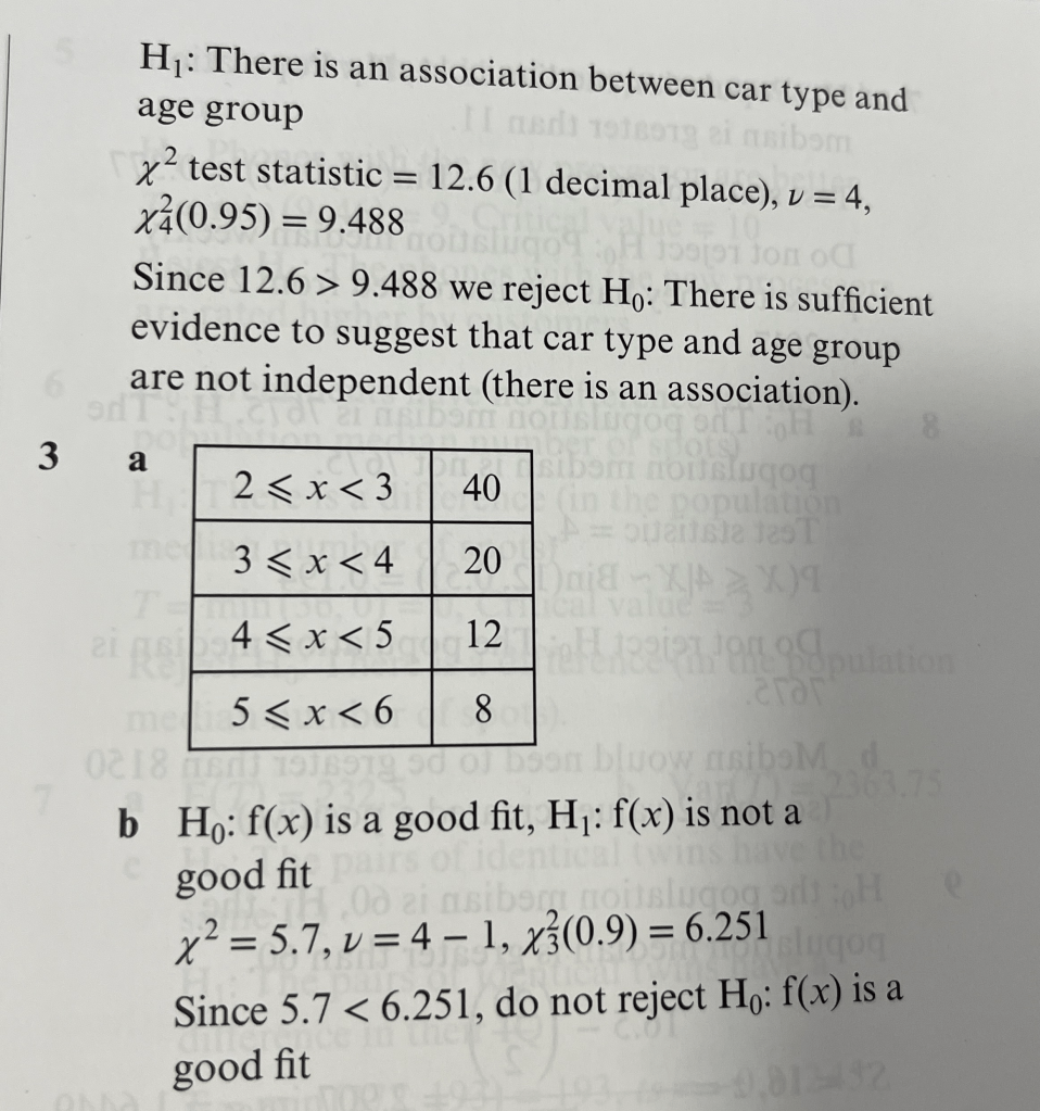
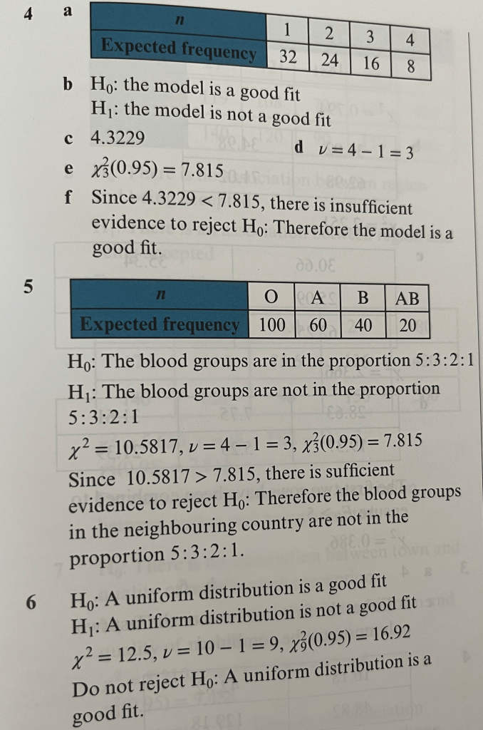
Answers to Exercise 2

Worked Solutions to Exercise 2

Goodness of Fit for Continuous Distributions

With continuous distributions, we need to look carefully at how the data are grouped in order to correctly calculate the expected values, as we will see in the following worked examples. If necessary, we can use $\bar{x}$ as an estimator for 𝝻 and s² as an estimate for 𝞂², each of which will reduced the degrees of freedom by 1.

Worked Example Normal Distribution

The weights of 150 newborn babies are are recorded to 1 decimal place in the following table.

Weight (kg)	2.0 – 2.4	2.5 – 2.9	3.0 – 3.4	3.5 – 3.9	4.0 – 4.4	4.5 -4.9
Frequency	8	14	54	43	22	9

It is believed that the data follow a normal distribution with variance 0.4. Test this belief at the 10% significance level.

In the next example we will consider a continuous uniform distribution (sometime known as a rectangular distribution based on the shape of its probability density function). Over the interval from a to b, this distribution has a PDF defined as $f(x) = \frac{1}{b-a}$ ∀ a ≤ x ≤ b and f(x) = 0 otherwise.

Worked Example. Continuous uniform Distribution

The time that people spend waiting for a bus is observed over 120 days and the results noted:

Time, t (minutes)	0-	10-	20-	30-	40-	50-60
Frequency	14	25	27	25	15	14

The departure time of the previous bus is unknown in each case. It is believed that the waiting times are uniformly distributed over one hour. Test this claim at the 10% level of significance.

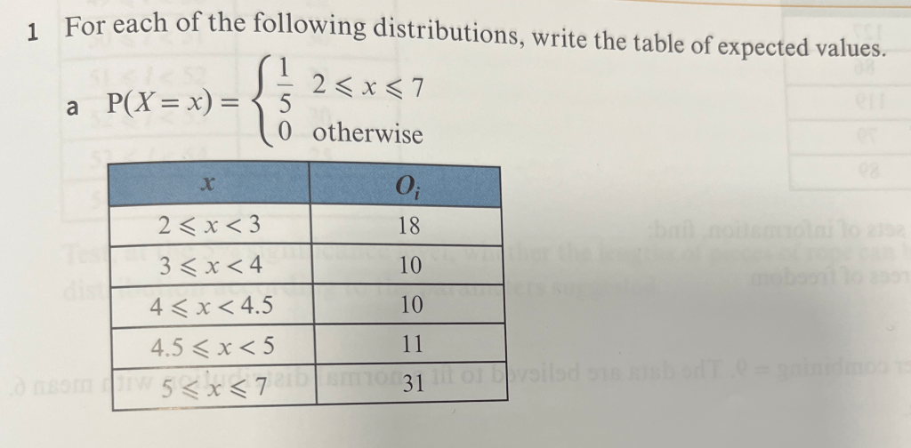
Exercise 3

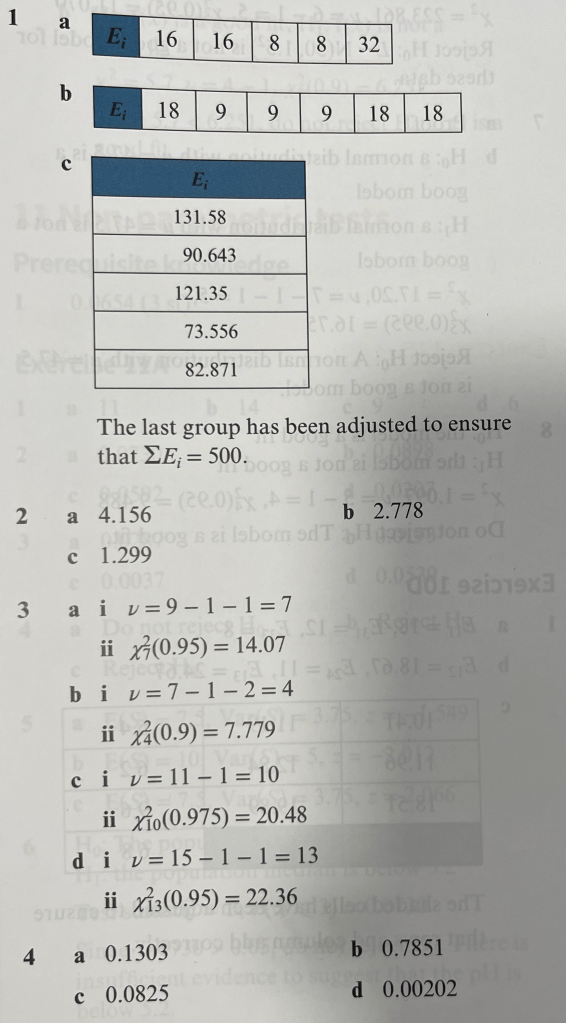
Answers to Exercise 3

Worked Solutions to Exercise 3

Testing Association using Contingency Tables

We can also use the chi-squared distribution to look for an association between two criteria (e.g. eye colour and hair colour). We must be able to put the data into a contingency table, as illustrated below:

		Hair Colour	Hair Colour	Hair Colour
		Brown	Blonde	Red	Row Totals
Eye Colour	Brown	63	31	6	R₁ = 100
Eye Colour	Blue	26	20	14	R₂ = 60
Eye Colour	Green	11	19	10	R₃ = 40
	Column Totals	C₁= 100	C₂ = 70	C₃ =30	T = 200

The contingency table shows the observed values. To calculate the expected values in each of the nine central cells, we use $E_{ij} = /frac{R_i \times C_j}{T}$ . As an example, lets use this to find the expected values for the above contingency table.

Because we know the totals, various of the internal numbers can be derived, which reduceds teh number of free independent variables. In general, the number of degrees of freedom of an mxn contingency table is 𝞶 = (m-1)(n-1)

Worked Example. Contingency Table Hypothesis Test

For the data below, conduct a hypothesis test at the 5% significance level to see if there is an association between eye colour and hair colour.

		Hair Colour	Hair Colour	Hair Colour
		Brown	Blonde	Red	Row Totals
Eye Colour	Brown	63	31	6	R₁ = 100
Eye Colour	Blue	26	20	14	R₂ = 60
Eye Colour	Green	11	19	10	R₃ = 40
	Column Totals	C₁= 100	C₂ = 70	C₃ =30	T = 200

Worked Example. Contingency Table Hypothesis Test 2

A research student collects information regarding the age of adults and the amount of debt that they have accumulated. The information collected is presented in the following table:

		Amount of debt	Amount of debt
		≤ $7500	> $7500
Age (years)	≤ 35	45	68
Age (years)	> 35	15	32

Test, at the 5% level of significance, to decide whether there is an association between age and amount of debt.

Worked Example. Contingency Table Hypothesis Test 3

In a school, the iGCSE results of 380 students are compared to see if there is an association between the grade in Mathematics and the grade in English. The results are shown in the table below:

		Mathematics Grade	Mathematics Grade	Mathematics Grade	Mathematics Grade	Mathematics Grade
		A	B	C	D	E
English Grade	A	33	23	9	4	1
English Grade	B	23	44	24	8	1
English Grade	C	14	30	28	11	2
English Grade	D	7	17	25	17	4
English Grade	E	1	6	19	22	7

(a.) Calculate a table of expected values.

(b.) Which columns would you combine and why?

(c.) Which rows might you consider combining? State the advantages and disadvantages of combining these rows.

(d.) Combining both rows and columns as suggested, perform a test, at the 1% significance level, to see whether there is an association between the grades achieved in English and in Maths.

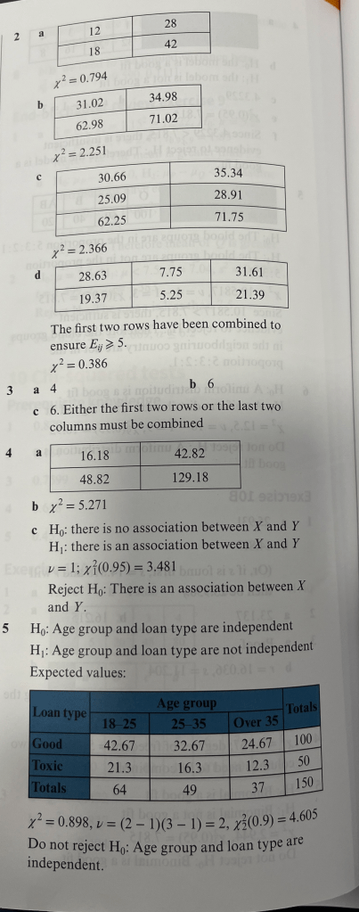
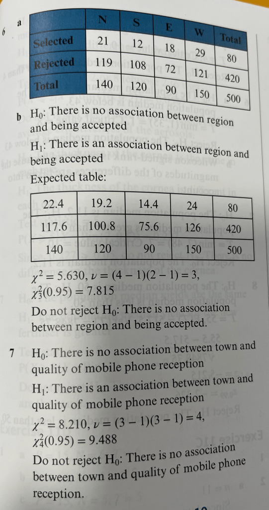
Exercise 4